Extra: The farmer’s problem and its variants

The Farmer’s Problem is a teaching example presented in the well-known textbook by John Birge and Francois Louveaux.

• Birge, John R., and Francois Louveaux. Introduction to stochastic programming. Springer Science & Business Media, 2011.

Preamble: Install Pyomo and a solver

The following cell sets and verifies a global SOLVER for the notebook. If run on Google Colab, the cell installs Pyomo and the HiGHS solver, while, if run elsewhere, it assumes Pyomo and HiGHS have been previously installed. It then sets to use HiGHS as solver via the appsi module and a test is performed to verify that it is available. The solver interface is stored in a global object SOLVER for later use.

import sys
 
if 'google.colab' in sys.modules:
    %pip install pyomo >/dev/null 2>/dev/null
    %pip install highspy >/dev/null 2>/dev/null

solver = 'appsi_highs'
 
import pyomo.environ as pyo
SOLVER = pyo.SolverFactory(solver)

assert SOLVER.available(), f"Solver {solver} is not available."

import numpy as np
import pandas as pd
import matplotlib.pyplot as plt
import pyomo.environ as pyo

Problem Statement

In the farmer’s problem, a European farmer must allocate 500 acres of land among three different crops (wheat, corn, and sugar beets) aiming to maximize profit. The following information is given:

• Planting one acre of wheat, corn and beet costs 150, 230 and 260 euro, respectively.

• The mean yields are 2.5, 3.0, and 20.0 tons per acre for wheat, corn, and sugar beets, respectively. The yields can vary up to 20% from nominal conditions depending on weather.

• At least 200 tons of wheat and 240 tons of corn are needed for cattle feed. Cattle feed can be raised on the farm or purchased from a wholesaler.

• The mean selling prices have been \\(170 and \\\)150 per ton of wheat and corn, respectively, over the last decade. The purchase prices are 40% more due to wholesaler’s margins and transportation costs.

• Sugar beets are a profitable crop expected to sell at 36 euro per ton, but there is a quota on sugar beet production. Any amount in excess of the quota can be sold at only 10 euro per ton. The farmer’s quota for next year is 6,000 tons.

Create three solutions for the farmer to consider.

1. How should the farmer allocate land to maximize profit for the mean weather conditions?

2. The second solution should explicitly consider the impact of weather. How should the farmer allocate land to maximize expected profit if the yields could go up or down by 20% due to weather conditions? What is the profit under each scenario?

3. During your interview you learned the farmer needs a minimal profit each year to stay in business. How would you allocate land use to maximize the worst case profit?

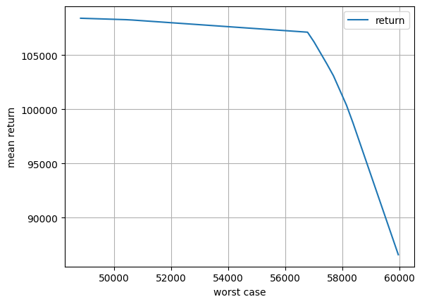
4. Determine the tradeoff between risk and return by computing the mean expected profit when the minimum required profit is the worst case found in part 3, and \\(58,000, \\\)56,000, \\(54,000, \\\)52,000, \\(50,000, and \\\)48,000. Compare these solutions to part 2 by plotting the expected loss in profit.

5. What would be your advice to the farmer regarding land allocation?

Data Summary

Scenario	Yield for wheat (tons/acre)	Yield for corn (tons/acre)	Yield for beets (tons/acre)
Good weather	3	3.6	24
Average weather	2.5	3	20
Bad weather	2	2.4	16

We first consider the case in which all the prices are fixed and not weather-dependent. The following table summarizes the data.

Commodity	Sell Price (euro/ton)	Market Demand (tons)	Excess Price	Buy Price (euro/ton)	Cattle Feed Required (tons)	Planting Cost (euro/acre)
Wheat	170	-	_	238	200	150
Corn	150	-	-	210	240	230
Beets	36	6000	10	0	-	260

Data Modeling

yields = pd.DataFrame(
    {
        "good": {"wheat": 3.0, "corn": 3.6, "beets": 24},
        "average": {"wheat": 2.5, "corn": 3.0, "beets": 20},
        "poor": {"wheat": 2.0, "corn": 2.4, "beets": 16},
    }
).T
display(yields)

	wheat	corn	beets
good	3.0	3.6	24.0
average	2.5	3.0	20.0
poor	2.0	2.4	16.0

crops = pd.DataFrame(
    {
        "wheat": {
            "planting cost": 150,
            "sell": 170,
            "buy": 238,
            "required": 200,
        },
        "corn": {
            "planting cost": 230,
            "sell": 150,
            "buy": 210,
            "required": 240,
        },
        "beets": {
            "planting cost": 260,
            "sell": 36,
            "quota": 6000,
            "excess": 10,
        },
    }
).T

# fill NaN

bigM = 20000
crops["buy"].fillna(bigM, inplace=True)
crops["quota"].fillna(bigM, inplace=True)
crops["required"].fillna(0, inplace=True)
crops["excess"].fillna(0, inplace=True)

display(crops)

	planting cost	sell	buy	required	quota	excess
wheat	150.0	170.0	238.0	200.0	20000.0	0.0
corn	230.0	150.0	210.0	240.0	20000.0	0.0
beets	260.0	36.0	20000.0	0.0	6000.0	10.0

Model Building

def farmer(crops, yields, total_land=500):
    m = pyo.ConcreteModel("Farmer's Problem")

    m.CROPS = pyo.Set(initialize=crops.index)
    m.SCENARIOS = pyo.Set(initialize=yields.index)

    # first stage variables
    m.acres = pyo.Var(m.CROPS, bounds=(0, total_land))

    # second stage variables (all units in tons)
    bounds = (0, yields.max().max() * total_land)
    m.grow = pyo.Var(m.SCENARIOS, m.CROPS, bounds=bounds)
    m.buy = pyo.Var(m.SCENARIOS, m.CROPS, bounds=bounds)
    m.sell = pyo.Var(m.SCENARIOS, m.CROPS, bounds=bounds)
    m.excess = pyo.Var(m.SCENARIOS, m.CROPS, bounds=bounds)

    # first stage model
    @m.Constraint()
    def limit_on_planted_land(m):
        return pyo.summation(m.acres) <= total_land

    # second stage model
    @m.Constraint(m.SCENARIOS, m.CROPS)
    def crop_yield(m, s, c):
        return m.grow[s, c] == yields.loc[s, c] * m.acres[c]

    @m.Constraint(m.SCENARIOS, m.CROPS)
    def balance(m, s, c):
        return (
            m.grow[s, c] + m.buy[s, c]
            == m.sell[s, c] + crops.loc[c, "required"] + m.excess[s, c]
        )

    @m.Disjunction(m.SCENARIOS, m.CROPS, xor=True)
    def quota(m, s, c):
        under_quota = [
            m.grow[s, c] <= crops.loc[c, "quota"],
            m.excess[s, c] == 0,
        ]
        over_quota = [
            m.grow[s, c] >= crops.loc[c, "quota"],
            m.sell[s, c] <= crops.loc[c, "quota"],
        ]
        return [under_quota, over_quota]

    # expressions for objective functions
    @m.Expression(m.SCENARIOS, m.CROPS)
    def expense(m, s, c):
        return (
            crops.loc[c, "planting cost"] * m.acres[c]
            + crops.loc[c, "buy"] * m.buy[s, c]
        )

    @m.Expression(m.SCENARIOS, m.CROPS)
    def revenue(m, s, c):
        return (
            crops.loc[c, "sell"] * m.sell[s, c]
            + crops.loc[c, "excess"] * m.excess[s, c]
        )

    @m.Expression(m.SCENARIOS)
    def scenario_profit(m, s):
        return sum(m.revenue[s, c] - m.expense[s, c] for c in m.CROPS)

    return m

def farm_report(m):
    print(f"Objective = {m.objective():0.2f}")
    for s in m.SCENARIOS:
        print(f"\nScenario: {s}")
        print(f"Scenario profit = {m.scenario_profit[s]()}")
        df = pd.DataFrame()
        df["plant [acres]"] = pd.Series({c: m.acres[c]() for c in m.CROPS})
        df["grow [tons]"] = pd.Series({c: m.grow[s, c]() for c in m.CROPS})
        df["buy [tons]"] = pd.Series({c: m.buy[s, c]() for c in m.CROPS})
        df["feed [tons]"] = pd.Series({c: crops.loc[c, "required"] for c in m.CROPS})
        df["quota [tons]"] = pd.Series({c: crops.loc[c, "quota"] for c in m.CROPS})
        df["sell [tons]"] = pd.Series({c: m.sell[s, c]() for c in m.CROPS})
        df["excess [tons]"] = pd.Series({c: m.excess[s, c]() for c in m.CROPS})
        df["revenue [euro]"] = pd.Series({c: m.revenue[s, c]() for c in m.CROPS})
        df["expense [euro]"] = pd.Series({c: m.expense[s, c]() for c in m.CROPS})
        df["profit [euro]"] = pd.Series(
            {c: m.revenue[s, c]() - m.expense[s, c]() for c in m.CROPS}
        )
        display(df.round(2))

1. Mean Solution

m = farmer(crops, pd.DataFrame(yields.mean(), columns=["mean"]).T)
pyo.TransformationFactory("gdp.bigm").apply_to(m)


@m.Objective(sense=pyo.maximize)
def objective(m):
    return pyo.summation(m.scenario_profit)


SOLVER.solve(m)
farm_report(m)

Objective = 118600.00

Scenario: mean
Scenario profit = 118599.99999999997

	plant [acres]	grow [tons]	buy [tons]	feed [tons]	quota [tons]	sell [tons]	excess [tons]	revenue [euro]	expense [euro]	profit [euro]
wheat	120.0	300.0	0.0	200.0	20000.0	100.0	0.0	17000.0	18000.0	-1000.0
corn	80.0	240.0	0.0	240.0	20000.0	0.0	0.0	0.0	18400.0	-18400.0
beets	300.0	6000.0	0.0	0.0	6000.0	6000.0	0.0	216000.0	78000.0	138000.0

2. Stochastic Solution

The problem statement asks for a number of different analyses. In a consulting situation, it is possible the client would ask more “what if” questions after hearing the initial results. For these reasons, we build a function that returns a Pyomo model the variables and expressions needed to address all parts of the problem.

# maximize mean profit
m = farmer(crops, yields)
pyo.TransformationFactory("gdp.bigm").apply_to(m)


@m.Objective(sense=pyo.maximize)
def objective(m):
    return pyo.summation(m.scenario_profit) / len(m.SCENARIOS)


SOLVER.solve(m)
farm_report(m)

Objective = 108390.00

Scenario: good
Scenario profit = 167000.0

	plant [acres]	grow [tons]	buy [tons]	feed [tons]	quota [tons]	sell [tons]	excess [tons]	revenue [euro]	expense [euro]	profit [euro]
wheat	170.0	510.0	0.0	200.0	20000.0	310.0	0.0	52700.0	25500.0	27200.0
corn	80.0	288.0	0.0	240.0	20000.0	48.0	0.0	7200.0	18400.0	-11200.0
beets	250.0	6000.0	0.0	0.0	6000.0	6000.0	0.0	216000.0	65000.0	151000.0

Scenario: average
Scenario profit = 109350.0

	plant [acres]	grow [tons]	buy [tons]	feed [tons]	quota [tons]	sell [tons]	excess [tons]	revenue [euro]	expense [euro]	profit [euro]
wheat	170.0	425.0	0.0	200.0	20000.0	225.0	0.0	38250.0	25500.0	12750.0
corn	80.0	240.0	0.0	240.0	20000.0	0.0	0.0	0.0	18400.0	-18400.0
beets	250.0	5000.0	0.0	0.0	6000.0	5000.0	0.0	180000.0	65000.0	115000.0

Scenario: poor
Scenario profit = 48820.0

	plant [acres]	grow [tons]	buy [tons]	feed [tons]	quota [tons]	sell [tons]	excess [tons]	revenue [euro]	expense [euro]	profit [euro]
wheat	170.0	340.0	0.0	200.0	20000.0	140.0	0.0	23800.0	25500.0	-1700.0
corn	80.0	192.0	48.0	240.0	20000.0	0.0	0.0	0.0	28480.0	-28480.0
beets	250.0	4000.0	0.0	0.0	6000.0	4000.0	0.0	144000.0	65000.0	79000.0

3. Worst Case Solution

# find worst case profit
m = farmer(crops, yields)
pyo.TransformationFactory("gdp.bigm").apply_to(m)

m.worst_case_profit = pyo.Var()


@m.Constraint(m.SCENARIOS)
def lower_bound_profit(m, s):
    return m.worst_case_profit <= m.scenario_profit[s]


@m.Objective(sense=pyo.maximize)
def objective(m):
    return m.worst_case_profit


SOLVER.solve(m)
farm_report(m)

Objective = 59950.00

Scenario: good
Scenario profit = 59950.0

	plant [acres]	grow [tons]	buy [tons]	feed [tons]	quota [tons]	sell [tons]	excess [tons]	revenue [euro]	expense [euro]	profit [euro]
wheat	100.0	300.0	0.0	200.0	20000.0	100.0	0.0	17000.0	15000.0	2000.0
corn	25.0	90.0	150.0	240.0	20000.0	0.0	0.0	0.0	37250.0	-37250.0
beets	375.0	9000.0	0.0	0.0	6000.0	3950.0	5050.0	192700.0	97500.0	95200.0

Scenario: average
Scenario profit = 86599.99999999997

	plant [acres]	grow [tons]	buy [tons]	feed [tons]	quota [tons]	sell [tons]	excess [tons]	revenue [euro]	expense [euro]	profit [euro]
wheat	100.0	250.0	0.0	200.0	20000.0	50.0	0.0	8500.0	15000.0	-6500.0
corn	25.0	75.0	165.0	240.0	20000.0	0.0	0.0	0.0	40400.0	-40400.0
beets	375.0	7500.0	0.0	0.0	6000.0	6000.0	1500.0	231000.0	97500.0	133500.0

Scenario: poor
Scenario profit = 59950.0

	plant [acres]	grow [tons]	buy [tons]	feed [tons]	quota [tons]	sell [tons]	excess [tons]	revenue [euro]	expense [euro]	profit [euro]
wheat	100.0	200.0	0.0	200.0	20000.0	0.0	0.0	0.0	15000.0	-15000.0
corn	25.0	60.0	180.0	240.0	20000.0	0.0	0.0	0.0	43550.0	-43550.0
beets	375.0	6000.0	0.0	0.0	6000.0	6000.0	0.0	216000.0	97500.0	118500.0

worst_case_profit = m.worst_case_profit()

# maximize expected profit subject to worst case as lower bound

m = farmer(crops, yields)
pyo.TransformationFactory("gdp.bigm").apply_to(m)


@m.Constraint(m.SCENARIOS)
def lower_bound_profit(m, s):
    return worst_case_profit <= m.scenario_profit[s]


@m.Objective(sense=pyo.maximize)
def objective(m):
    return pyo.summation(m.scenario_profit) / len(m.SCENARIOS)


SOLVER.solve(m)
farm_report(m)

Objective = 86600.00

Scenario: good
Scenario profit = 113250.0

	plant [acres]	grow [tons]	buy [tons]	feed [tons]	quota [tons]	sell [tons]	excess [tons]	revenue [euro]	expense [euro]	profit [euro]
wheat	100.0	300.0	0.0	200.0	20000.0	100.0	0.0	17000.0	15000.0	2000.0
corn	25.0	90.0	150.0	240.0	20000.0	0.0	0.0	0.0	37250.0	-37250.0
beets	375.0	9000.0	0.0	0.0	6000.0	6000.0	3000.0	246000.0	97500.0	148500.0

Scenario: average
Scenario profit = 86600.0

	plant [acres]	grow [tons]	buy [tons]	feed [tons]	quota [tons]	sell [tons]	excess [tons]	revenue [euro]	expense [euro]	profit [euro]
wheat	100.0	250.0	0.0	200.0	20000.0	50.0	0.0	8500.0	15000.0	-6500.0
corn	25.0	75.0	165.0	240.0	20000.0	0.0	0.0	0.0	40400.0	-40400.0
beets	375.0	7500.0	0.0	0.0	6000.0	6000.0	1500.0	231000.0	97500.0	133500.0

Scenario: poor
Scenario profit = 59950.0

	plant [acres]	grow [tons]	buy [tons]	feed [tons]	quota [tons]	sell [tons]	excess [tons]	revenue [euro]	expense [euro]	profit [euro]
wheat	100.0	200.0	0.0	200.0	20000.0	0.0	0.0	0.0	15000.0	-15000.0
corn	25.0	60.0	180.0	240.0	20000.0	0.0	0.0	0.0	43550.0	-43550.0
beets	375.0	6000.0	0.0	0.0	6000.0	6000.0	0.0	216000.0	97500.0	118500.0

4. Risk versus Return

df = pd.DataFrame()

for wc in np.linspace(48820, 59950, 50):
    m = farmer(crops, yields)
    pyo.TransformationFactory("gdp.bigm").apply_to(m)

    @m.Constraint(m.SCENARIOS)
    def min_profit(m, s):
        return m.scenario_profit[s] >= wc

    # maximize mean profit
    @m.Objective(sense=pyo.maximize)
    def objective(m):
        return pyo.summation(m.scenario_profit) / len(m.SCENARIOS)

    SOLVER.solve(m)

    df.loc[wc, "return"] = m.objective()
    df.loc[wc, "wc"] = wc

df.plot(x="wc", y="return", xlabel="worst case", ylabel="mean return", grid=True)

<Axes: xlabel='worst case', ylabel='mean return'>

5. Recommended Planting Strategy

df = pd.DataFrame()

for wc in np.linspace(56750, 56820, 50):
    m = farmer(crops, yields)
    pyo.TransformationFactory("gdp.bigm").apply_to(m)

    @m.Constraint(m.SCENARIOS)
    def min_profit(m, s):
        return m.scenario_profit[s] >= wc

    # maximize mean profit
    @m.Objective(sense=pyo.maximize)
    def objective(m):
        return pyo.summation(m.scenario_profit) / len(m.SCENARIOS)

    SOLVER.solve(m)

    df.loc[wc, "return"] = m.objective()
    df.loc[wc, "wc"] = wc

df.plot(x="wc", y="return", xlabel="worst case", ylabel="mean return", grid=True)

<Axes: xlabel='worst case', ylabel='mean return'>

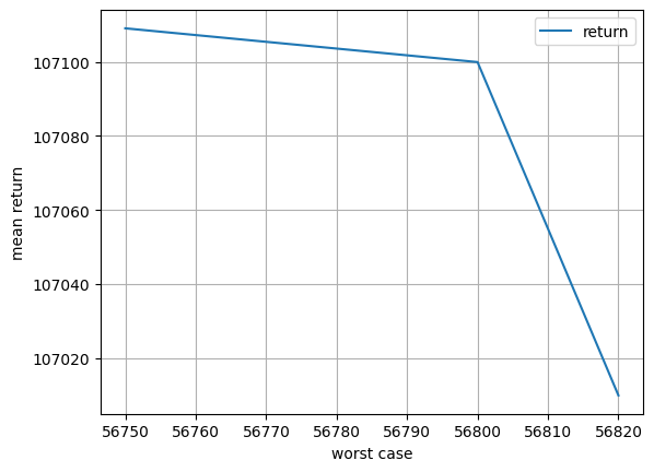
What we see is that the worst case can be raised from 48,820 to 56,800 (a difference of 7,980 euro) at a cost of reducing the expected from from 108,390 to 107,100 (a reduction of 1,290 euro). This improvement in worst-case performance may be worth the reduction in mean profit.

wc = 56800

m = farmer(crops, yields)
pyo.TransformationFactory("gdp.bigm").apply_to(m)


@m.Constraint(m.SCENARIOS)
def min_profit(m, s):
    return m.scenario_profit[s] >= wc


# maximize mean profit
@m.Objective(sense=pyo.maximize)
def objective(m):
    return pyo.summation(m.scenario_profit) / len(m.SCENARIOS)


SOLVER.solve(m)

farm_report(m)

Objective = 107100.00

Scenario: good
Scenario profit = 147000.0

	plant [acres]	grow [tons]	buy [tons]	feed [tons]	quota [tons]	sell [tons]	excess [tons]	revenue [euro]	expense [euro]	profit [euro]
wheat	100.0	300.0	0.0	200.0	20000.0	100.0	0.0	17000.0	15000.0	2000.0
corn	100.0	360.0	0.0	240.0	20000.0	120.0	0.0	18000.0	23000.0	-5000.0
beets	300.0	7200.0	0.0	0.0	6000.0	6000.0	1200.0	228000.0	78000.0	150000.0

Scenario: average
Scenario profit = 117499.99999999999

	plant [acres]	grow [tons]	buy [tons]	feed [tons]	quota [tons]	sell [tons]	excess [tons]	revenue [euro]	expense [euro]	profit [euro]
wheat	100.0	250.0	0.0	200.0	20000.0	50.0	0.0	8500.0	15000.0	-6500.0
corn	100.0	300.0	0.0	240.0	20000.0	60.0	0.0	9000.0	23000.0	-14000.0
beets	300.0	6000.0	0.0	0.0	6000.0	6000.0	0.0	216000.0	78000.0	138000.0

Scenario: poor
Scenario profit = 56799.999999999956

	plant [acres]	grow [tons]	buy [tons]	feed [tons]	quota [tons]	sell [tons]	excess [tons]	revenue [euro]	expense [euro]	profit [euro]
wheat	100.0	200.0	0.0	200.0	20000.0	-0.0	0.0	0.0	15000.0	-15000.0
corn	100.0	240.0	0.0	240.0	20000.0	0.0	0.0	0.0	23000.0	-23000.0
beets	300.0	4800.0	0.0	0.0	6000.0	4800.0	0.0	172800.0	78000.0	94800.0

Bibliographic Notes

The Farmer’s Problem is well known in the stochastic programming community. Examples of treatments include the following web resources:

• http://user.engineering.uiowa.edu/~dbricker/stacks_pdf1/slpwr_farmer.pdf

• https://www.math.uh.edu/~rohop/Spring_15/Chapter1.pdf