5.2 Ordinary Least Squares (OLS) Regression

In Chapter 2 we introduced linear regression with least absolute deviations (LAD), see this notebook. Here we consider the same problem setting, but slightly change the underlying optimization problem, in particular its objective function, obtaining the classical ordinary least squares (OLS) regression.

Preamble: Install Pyomo and a solver

This cell selects and verifies a global SOLVER for the notebook. If run on Google Colab, the cell installs Pyomo and ipopt, then sets SOLVER to use the ipopt solver. If run elsewhere, it assumes Pyomo and the Mosek solver have been previously installed and sets SOLVER to use the Mosek solver via the Pyomo SolverFactory. It then verifies that SOLVER is available. For linear problems, the solver HiGHS is imported and used.

import sys, os

if 'google.colab' in sys.modules:
    %pip install idaes-pse --pre >/dev/null 2>/dev/null
    %pip install highspy >/dev/null 2>/dev/null
    !idaes get-extensions --to ./bin 
    os.environ['PATH'] += ':bin'
    solver = 'ipopt'
else:
    solver = 'mosek_direct'

import pyomo.environ as pyo
SOLVER = pyo.SolverFactory(solver)
assert SOLVER.available(), f"Solver {solver} is not available."

solver_LO = 'appsi_highs'
SOLVER_LO = pyo.SolverFactory(solver_LO)
assert SOLVER_LO.available(), f"Solver {solver_LO} is not available."

Generate data

The Python scikit learn library for machine learning provides a full-featured collection of tools for regression. The following cell uses make_regression from scikit learn to generate a synthetic data set for use in subsequent cells. The data consists of a numpy array y containing n_samples of one dependent variable \(y\), and an array X containing n_samples observations of n_features independent explanatory variables.

from sklearn.datasets import make_regression
import numpy as np
import matplotlib.pyplot as plt
import pyomo.environ as pyo

n_features = 1
n_samples = 500
noise = 75

# generate regression dataset
np.random.seed(2022)
X, y = make_regression(n_samples=n_samples, n_features=n_features, noise=noise)

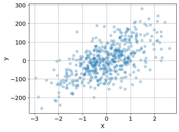
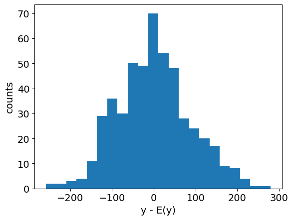
Data Visualization

Before going further, it is generally useful to prepare an initial visualization of the data. The following cell presents a scatter plot of \(y\) versus \(x\) for the special case of one explanatory variable, and a histogram of the difference between \(y\) and the mean value \(\bar{y}\). This histogram will provide a reference against which to compare the residual error in \(y\) after regression.

if n_features == 1:
    plt.scatter(X, y, alpha=0.3)
    plt.xlabel("X")
    plt.ylabel("y")
    plt.grid(True)

plt.figure()
plt.hist(y - np.mean(y), bins=int(np.sqrt(len(y))))
plt.xlabel("y - E(y)")
plt.ylabel("counts")
plt.show()

OLS regression as an optimization model

Similarly to the LAD regression example, suppose we have a finite data set consisting of \(n\) points \(\{({X}^{(i)}, y^{(i)})\}_{i=1,\dots,n}\) with \({X}^{(i)} \in \mathbb R^k\) and \(y^{(i)} \in \mathbb R\). We want to fit a linear model with intercept, whose error or deviation term \(e_i\) is equal to

\[ e_i = y^{(i)} - {m}^\top {X}^{(i)} - b = y^{(i)} - \sum_{j=1}^k X^{(i)}_j m_j - b, \]

for some real numbers \(b, m_1,\dots,m_k\). The Ordinary Least Squares (OLS) is a possible statistical optimality criterion for such a linear regression, which tries to minimize the sum of the errors squares, that is \(\sum_{i=1}^n e_i^2\). The OLS regression can thus be formulated as an optimization with the coefficients \(b\) and \(m_i\)’s and the errors \(e_i\)’s as the decision variables, namely

\[\begin{split} \begin{align} \min \quad & \sum_{i=1}^n e_i^2\\ \text{s.t.} \quad & e_i = y^{(i)} - {m}^\top {X}^{(i)} - b, \qquad \forall\, i=1,\dots,n. \end{align} \end{split}\]

Convexity of the optimization model

Denote by \({\theta}=(b,{m}) \in \mathbb{R}^{k+1}\) the vector comprising all variables, by \(y =(y^{(1)}, \dots, y^{(n)})\), and by \({\tilde{X}} = \mathbb{R}^{d \times (n+1)}\) the so-called design matrix associated with the dataset, that is

\[ {\tilde{X}} = \left[ \begin{array}{cccc} {1} & {X}^{(1)} & \dots & {X}^{(n)} \end{array}\right]. \]

We can then rewrite the minimization problem above as an unconstrained optimization problem in the vector of variables \({\theta}\), namely

\[ \min_{{\theta}} f({\theta}), \]

with \(f: \mathbb{R}^{k+1} \rightarrow \mathbb{R}\) defined as \(f({\theta}):=\| {y} - {\tilde{X}} {\theta} \|_2^2\). Note that here \(y\) and \({X}^{(i)}\), \(i=1,\dots,n\) are not a vector of variables, but rather of known parameters. The Hessian of the objective function can be calculated to be

\[ \nabla^2 f(\theta) = 2 {\tilde{X}}^\top {\tilde{X}}. \]

In particular, it is a constant matrix that does not depend on the variables \({\theta}\) and it is always positive semi-definite, since

\[ t^\top \nabla^2 f(\theta) t = 2 t^\top {\tilde{X}}^\top \tilde{X} t = 2 \| {\tilde{X}} t \|_2^2 \geq 0, \qquad \forall \, t \in \mathbb{R}^{k+1}. \]

The OLS optimization problem is then always convex.

The OLS problem can be implemented in Pyomo as follows. Leveraging the convexity of the problem and thus the uniqueness of the solution, in case mosek is not available, we could resort to the generic nonlinear solver ipopt.

def ols_regression(X, y):
    m = pyo.ConcreteModel("OLS Regression")

    n, k = X.shape

    # note use of Python style zero based indexing
    m.I = pyo.RangeSet(0, n - 1)
    m.J = pyo.RangeSet(0, k - 1)

    m.e = pyo.Var(m.I, domain=pyo.Reals)
    m.m = pyo.Var(m.J)
    m.b = pyo.Var()

    @m.Constraint(m.I)
    def residuals(m, i):
        return m.e[i] == y[i] - sum(X[i][j] * m.m[j] for j in m.J) - m.b

    @m.Objective(sense=pyo.minimize)
    def sum_of_square_errors(m):
        return sum((m.e[i]) ** 2 for i in m.I)

    return m


m = ols_regression(X, y)
SOLVER.solve(m)
m.m.display()
m.b.display()

m : Size=1, Index=J
    Key : Lower : Value              : Upper : Fixed : Stale : Domain
      0 :  None : 53.498473126416755 :  None : False : False :  Reals
b : Size=1, Index=None
    Key  : Lower : Value             : Upper : Fixed : Stale : Domain
    None :  None : 0.428094680287527 :  None : False : False :  Reals

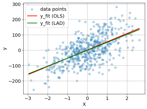
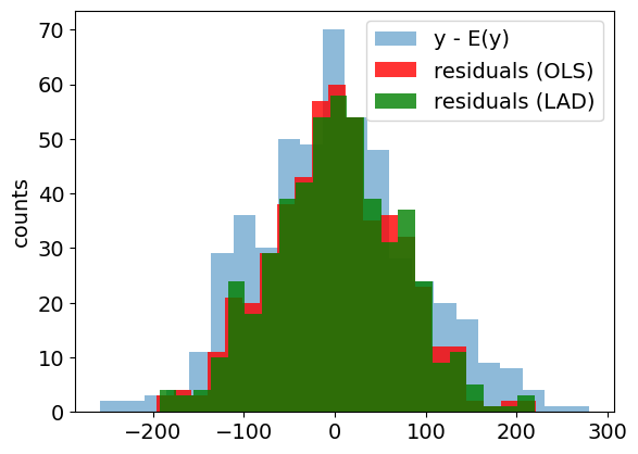
Visualizing the results and comparison with LAD regression

def lad_regression(X, y):
    m = pyo.ConcreteModel("LAD Regression")

    n, k = X.shape

    # note use of Python style zero based indexing
    m.I = pyo.RangeSet(0, n - 1)
    m.J = pyo.RangeSet(0, k - 1)

    m.ep = pyo.Var(m.I, domain=pyo.NonNegativeReals)
    m.em = pyo.Var(m.I, domain=pyo.NonNegativeReals)
    m.m = pyo.Var(m.J)
    m.b = pyo.Var()

    @m.Constraint(m.I)
    def residuals(m, i):
        return m.ep[i] - m.em[i] == y[i] - sum(X[i][j] * m.m[j] for j in m.J) - m.b

    @m.Objective(sense=pyo.minimize)
    def sum_of_abs_errors(m):
        return sum(m.ep[i] + m.em[i] for i in m.I)

    return m


m2 = lad_regression(X, y)
SOLVER_LO.solve(m2)
m2.m.display()
m2.b.display()

m : Size=1, Index=J
    Key : Lower : Value     : Upper : Fixed : Stale : Domain
      0 :  None : 51.428576 :  None : False : False :  Reals
b : Size=1, Index=None
    Key  : Lower : Value      : Upper : Fixed : Stale : Domain
    None :  None : -1.4130268 :  None : False : False :  Reals

y_fit = np.array([sum(x[j] * m.m[j]() for j in m.J) + m.b() for x in X])
y_fit2 = np.array([sum(x[j] * m2.m[j]() for j in m2.J) + m2.b() for x in X])

plt.rcParams.update({"font.size": 14})

if n_features == 1:
    plt.scatter(X, y, alpha=0.3, label="data points")
    plt.plot(X, y_fit, "r", label="y_fit (OLS)", lw=2)
    plt.plot(X, y_fit2, "g", label="y_fit (LAD)", lw=2)
    plt.xlabel("X")
    plt.ylabel("y")
    plt.grid(True)
    plt.legend()
    plt.tight_layout()
    plt.savefig("ols-regression.svg", dpi=300, bbox_inches="tight")

plt.figure()
plt.hist(y - np.mean(y), bins=int(np.sqrt(len(y))), alpha=0.5, label="y - E(y)")
plt.hist(
    y - y_fit,
    bins=int(np.sqrt(len(y))),
    color="r",
    alpha=0.8,
    label="residuals (OLS)",
)
plt.hist(
    y - y_fit2,
    bins=int(np.sqrt(len(y))),
    color="g",
    alpha=0.8,
    label="residuals (LAD)",
)
plt.ylabel("counts")
plt.legend()
plt.show()