
1.2 A basic Pyomo model#
Pyomo is an algebraic modeling language for mathematical optimization that is integrated within the Python programming environment. It enables users to create optimization models consisting of decision variables, expressions, objective functions, and constraints. Pyomo provides tools to transform models, and then solve them using a variety of open-source and commercial solvers. As an open-source project, Pyomo is not tied to any specific vendor, solver, or class of mathematical optimization problems, and is constantly evolving through contributions from third-party developers.
This notebook introduces basic elements of Pyomo common to most applications for the small production planning problem introduced earlier in this notebook introduced in a companion notebook:
The Pyomo model shown below is a direct translation of the mathematical model into basic Pyomo components. In this approach, parameter values from the mathematical model are included directly in the Pyomo model for simplicity. This method works well for problems with a few decision variables and constraints, but it limits the reuse of the model. Another notebook will demonstrate Pyomo features for writing models for more generic, “data-driven” applications.
This notebook also introduces the use of Python decorators to designate Pyomo expressions, objectives, and constraints. While decorators may be unfamiliar to some Python users, or even current Pyomo users, they offer a significant improvement in the readability of Pyomo model. This feature is relatively new and is available in recent versions of Pyomo.
Preamble: Install Pyomo and a solver#
This collection of notebooks is intended to be run in the cloud on Google Colab or on a personal computer. To meet this goal, we start each notebook by verifying the installation of Pyomo and an appropriate solver.
When run on Google Colab, an installation of Pyomo and a solver must be done for each new Colab session. The HiGHS solver is a high performance open source solver for linear and mixed integer optimization on Google Colab. For a personal computer, we assume Python, Pyomo and the HiGHS solver have been previously installed. Note that there are other suitable solvers, both open-source, such as COIN-OR Cbc solver and GLPK, and commercial, such as CPLEX, Gurobi, and Mosek.
The following cell sets and verifies a global SOLVER for the notebook. If run on Google Colab, the cell installs Pyomo and the HiGHS solver, while, if run elsewhere, it
assumes Pyomo and HiGHS have been previously installed. It then sets to use HiGHS as solver via the appsi module and a test is performed to verify that it is available. The solver interface is stored in a global object SOLVER for later use.
import sys

if 'google.colab' in sys.modules:
    %pip install pyomo >/dev/null 2>/dev/null
    %pip install highspy >/dev/null 2>/dev/null

solver = 'appsi_highs'

import pyomo.environ as pyo
SOLVER = pyo.SolverFactory(solver)

assert SOLVER.available(), f"Solver {solver} is not available."
Step 1. Import Pyomo#
The first step for a new Pyomo model is to import the needed components into the Python environment. The module pyomo.environ provides the components most commonly used for building Pyomo models. Although this module was imported in the previous code cell, we mention it again here also to emphasize our standardized conventions. Throughout this collection of notebooks, a uniform standard is maintained for importing pyomo.environ consistently using the alias pyo.
import pyomo.environ as pyo
Step 2. The ConcreteModel object#
Pyomo models can be named using any standard Python variable name. In the following code cell, an instance of ConcreteModel is created and stored in a Python variable named model. It is best to use a short name since it will appear as a prefix for every Pyomo variable and constraint. ConcreteModel accepts an optional string argument used to title subsequent reports.
pyo.ConcreteModel() is used to create a model object when the problem data is known at the time of construction. Alternatively, pyo.AbstractModel() can create models where the problem data will be provided later to create specific model instances. But this is normally not needed when using the “data-driven” approach demonstrated in this collection of notebooks.
# create model with optional problem title
model = pyo.ConcreteModel("Production Planning: Version 1")
The .display() method displays the current content of a Pyomo model. When developing new models, this is a useful tool to verify that the model is being constructed as intended. At this stage, the major components of the model are empty.
# display model
model.display()
Model 'Production Planning: Version 1'

  Variables:
    None

  Objectives:
    None

  Constraints:
    None
Step 3. Decision variables#
Decision variables are created with pyo.Var(). Decision variables can be assigned to any valid Python identifier. Here, we assign decision variables to the model instance using the Python ‘dot’ notation. The variable names are chosen to reflect their names in the mathematical model.
pyo.Var() accepts optional keyword arguments. The most commonly used keyword arguments are:
domainspecifies a set of values for a decision variable. By default, the domain is the set of all real numbers. Other commonly used domains arepyo.NonNegativeReals,pyo.NonNegativeIntegers, andpyo.Binary.boundsis an optional keyword argument to specify a tuple containing values for the lower and upper bounds. It is good modeling practice to specify any known and fixed bounds on the decision variables.Nonecan be used as a placeholder if one of the two bounds is unknown. Specifying the bounds as(0, None)is equivalent to specifying the domain aspyo.NonNegativeReals.
The use of the optional keywords is shown in the following cell. Displaying the model shows that the value of the decision variables is not yet known.
# create decision variables
model.x_M = pyo.Var(bounds=(0, None))
model.x_A = pyo.Var(bounds=(0, 80))
model.x_B = pyo.Var(bounds=(0, 100))

model.y_U = pyo.Var(bounds=(0, 40))
model.y_V = pyo.Var(bounds=(0, None))

# display updated model
model.display()
Model 'Production Planning: Version 1'

  Variables:
    x_M : Size=1, Index=None
        Key  : Lower : Value : Upper : Fixed : Stale : Domain
        None :     0 :  None :  None : False :  True :  Reals
    x_A : Size=1, Index=None
        Key  : Lower : Value : Upper : Fixed : Stale : Domain
        None :     0 :  None :    80 : False :  True :  Reals
    x_B : Size=1, Index=None
        Key  : Lower : Value : Upper : Fixed : Stale : Domain
        None :     0 :  None :   100 : False :  True :  Reals
    y_U : Size=1, Index=None
        Key  : Lower : Value : Upper : Fixed : Stale : Domain
        None :     0 :  None :    40 : False :  True :  Reals
    y_V : Size=1, Index=None
        Key  : Lower : Value : Upper : Fixed : Stale : Domain
        None :     0 :  None :  None : False :  True :  Reals

  Objectives:
    None

  Constraints:
    None
Step 4. Expressions#
Pyomo expressions are mathematical formulas that involve decision variables. The following cell creates expressions for revenue and cost that are assigned to model.revenue and model.cost, respectively.
# create expressions
model.revenue = 270 * model.y_U + 210 * model.y_V
model.cost = 10 * model.x_M + 50 * model.x_A + 40 * model.x_B

# expressions can be printed
print(model.revenue)
print(model.cost)
270*y_U + 210*y_V
10*x_M + 50*x_A + 40*x_B
Step 5. Objective#
The objective for this example is to maximize profit which is given by the difference between revenue and cost. There are two ways this objective could be specified in Pyomo.
The first method is to use pyo.Objective() where the expression to be optimized is assigned with the expr keyword and the type of objective is assigned with the sense keyword.
model.profit = pyo.Objective(expr=model.revenue - model.cost, sense=pyo.maximize)
Recent releases of Pyomo provide a second method that uses Python decorators to specify an objective. With a decorator, the same objective is written as
@model.Objective(sense=pyo.maximize)
def profit(m):
    return m.revenue - m.cost
Python decorators modify the behavior of the function defined in the next line. In this case, the decorator @model.Objective() modifies the behavior of profit() so that it returns an expression for the profit to Pyomo. The keyword sense sets the type of objective, which can either be to maximize or minimize the value returned by the objective function. The function profit(), after being decorated, takes the Pyomo model as its first argument and adds its name to the model attributes.
In effect, Pyomo decorators are tags that insert functions into a Pyomo model to serve as expressions, objectives, or constraints. Decorators can improve the readability and maintainability of more complex models. They also simplify the syntax for creating other Pyomo objects expressions, constraints, and other optimization-related elements.
Step 6. Constraints#
Constraints are logical relationships between expressions that define the range of feasible solutions in an optimization problem. A constraint consists of two expressions separated by one of the logical relationships. The logical relationships can be equality (==), less-than (<=), or greater-than (>=).
Constraints can be created with pyo.Constraint(). The constraint is passed as a keyword argument expr to pyo.Constraint(). For this application the constraints could be expressed as
    model.raw_materials = pyo.Constraint(expr = 10 * model.y_U + 9 * model.y_V <= model.x_M)
    model.labor_A = pyo.Constraint(expr = 1 * model.y_U + 1 * model.y_V <= model.x_A)
    model.labor_B = pyo.Constraint(expr = 2 * model.y_U + 1 * model.y_V <= model.x_B)
Alternatively, the @model.Constraint() decorator ‘tags’ the output of the following function as a constraint. For the present example, the constraints are expressed with decorators below. This collection of notebooks uses decorators whenever possible to improve the readability and maintainability of Pyomo models.
@model.Constraint()
def raw_materials(m):
    return 10 * m.y_U + 9 * m.y_V <= m.x_M


@model.Constraint()
def labor_A(m):
    return 1 * m.y_U + 1 * m.y_V <= m.x_A


@model.Constraint()
def labor_B(m):
    return 2 * m.y_U + 1 * m.y_V <= m.x_B


model.pprint()
5 Var Declarations
    x_A : Size=1, Index=None
        Key  : Lower : Value : Upper : Fixed : Stale : Domain
        None :     0 :  None :    80 : False :  True :  Reals
    x_B : Size=1, Index=None
        Key  : Lower : Value : Upper : Fixed : Stale : Domain
        None :     0 :  None :   100 : False :  True :  Reals
    x_M : Size=1, Index=None
        Key  : Lower : Value : Upper : Fixed : Stale : Domain
        None :     0 :  None :  None : False :  True :  Reals
    y_U : Size=1, Index=None
        Key  : Lower : Value : Upper : Fixed : Stale : Domain
        None :     0 :  None :    40 : False :  True :  Reals
    y_V : Size=1, Index=None
        Key  : Lower : Value : Upper : Fixed : Stale : Domain
        None :     0 :  None :  None : False :  True :  Reals

1 Objective Declarations
    profit : Size=1, Index=None, Active=True
        Key  : Active : Sense    : Expression
        None :   True : maximize : 270*y_U + 210*y_V - (10*x_M + 50*x_A + 40*x_B)

3 Constraint Declarations
    labor_A : Size=1, Index=None, Active=True
        Key  : Lower : Body            : Upper : Active
        None :  -Inf : y_U + y_V - x_A :   0.0 :   True
    labor_B : Size=1, Index=None, Active=True
        Key  : Lower : Body              : Upper : Active
        None :  -Inf : 2*y_U + y_V - x_B :   0.0 :   True
    raw_materials : Size=1, Index=None, Active=True
        Key  : Lower : Body                 : Upper : Active
        None :  -Inf : 10*y_U + 9*y_V - x_M :   0.0 :   True

9 Declarations: x_M x_A x_B y_U y_V profit raw_materials labor_A labor_B
Step 7. Solve the model#
With the model now fully specified, the next step is to compute a solution. A solver object is created with SolverFactory then applied to the model as shown in the following cell. The optional keyword tee=True causes the solver to print its output to the output. This can be useful for debugging problems that arise when developing a new model.
results = SOLVER.solve(model, tee=True)
Running HiGHS 1.5.3 [date: 2023-05-16, git hash: 594fa5a9d]
Copyright (c) 2023 HiGHS under MIT licence terms
WARNING: No semi-integer/integer variables in model with non-empty integrality
Presolving model
2 rows, 4 cols, 6 nonzeros
2 rows, 4 cols, 6 nonzeros
Presolve : Reductions: rows 2(-1); columns 4(-1); elements 6(-3)
Solving the presolved LP
Using EKK dual simplex solver - serial
  Iteration        Objective     Infeasibilities num(sum)
          0    -2.0999953995e+02 Ph1: 2(4); Du: 3(210) 0s
          3    -2.6000000000e+03 Pr: 0(0) 0s
Solving the original LP from the solution after postsolve
Model   status      : Optimal
Simplex   iterations: 3
Objective value     :  2.6000000000e+03
HiGHS run time      :          0.00
Step 8. Reporting the solution#
The final step in most applications is to report the solution in a suitable format. For this example, we demonstrate simple tabular and graphic reports using the Pandas library. For an overview of other ways to report and visualize the solutions, see also the appendix of this notebook from Chapter 4.
Pyomo pprint()#
Pyomo provides several functions for creating model reports that contain solution values. The pprint() method can be applied to the entire model, or to individual components of the model, as shown in the following cells.
# display the whole model
model.pprint()
5 Var Declarations
    x_A : Size=1, Index=None
        Key  : Lower : Value : Upper : Fixed : Stale : Domain
        None :     0 :  80.0 :    80 : False : False :  Reals
    x_B : Size=1, Index=None
        Key  : Lower : Value : Upper : Fixed : Stale : Domain
        None :     0 : 100.0 :   100 : False : False :  Reals
    x_M : Size=1, Index=None
        Key  : Lower : Value : Upper : Fixed : Stale : Domain
        None :     0 : 740.0 :  None : False : False :  Reals
    y_U : Size=1, Index=None
        Key  : Lower : Value : Upper : Fixed : Stale : Domain
        None :     0 :  20.0 :    40 : False : False :  Reals
    y_V : Size=1, Index=None
        Key  : Lower : Value : Upper : Fixed : Stale : Domain
        None :     0 :  60.0 :  None : False : False :  Reals

1 Objective Declarations
    profit : Size=1, Index=None, Active=True
        Key  : Active : Sense    : Expression
        None :   True : maximize : 270*y_U + 210*y_V - (10*x_M + 50*x_A + 40*x_B)

3 Constraint Declarations
    labor_A : Size=1, Index=None, Active=True
        Key  : Lower : Body            : Upper : Active
        None :  -Inf : y_U + y_V - x_A :   0.0 :   True
    labor_B : Size=1, Index=None, Active=True
        Key  : Lower : Body              : Upper : Active
        None :  -Inf : 2*y_U + y_V - x_B :   0.0 :   True
    raw_materials : Size=1, Index=None, Active=True
        Key  : Lower : Body                 : Upper : Active
        None :  -Inf : 10*y_U + 9*y_V - x_M :   0.0 :   True

9 Declarations: x_M x_A x_B y_U y_V profit raw_materials labor_A labor_B
# display a component of the model
model.profit.pprint()
profit : Size=1, Index=None, Active=True
    Key  : Active : Sense    : Expression
    None :   True : maximize : 270*y_U + 210*y_V - (10*x_M + 50*x_A + 40*x_B)
Accessing solution values with pyo.value()#
After a solution to a Pyomo model has been successfully computed, values for the objective, expressions, and decisions variables can be accessed with pyo.value().
pyo.value(model.profit)
2600.0
When combined with Python f strings, pyo.value() provides a convenient means of creating formatted reports.
print(f" Profit = {pyo.value(model.profit): 9.2f}")
print(f"Revenue = {pyo.value(model.revenue): 9.2f}")
print(f"   Cost = {pyo.value(model.cost): 9.2f}")
 Profit =   2600.00
Revenue =  18000.00
   Cost =  15400.00
Pyomo provides a shortcut notation for accessing solution. After a solution has been computed, a function with the same name as decision variable is created that will report the solution value.
print("x_A =", model.x_A())
print("x_B =", model.x_B())
print("x_M =", model.x_M())
x_A = 80.0
x_B = 100.0
x_M = 740.0
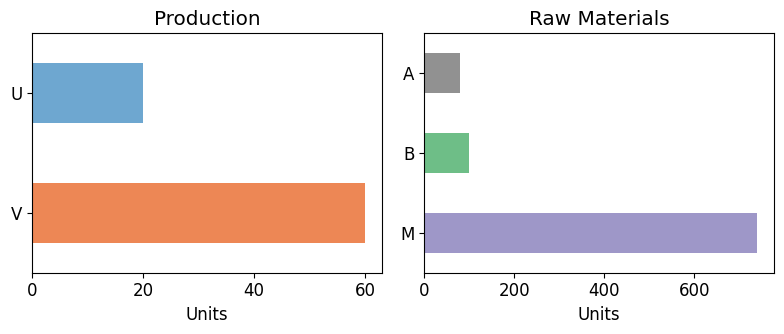
Creating reports with Pandas#
Pandas is an open-source library for working with data in Python and is widely used in the data science community. Here we use a Pandas Series() object to hold and display solution data. We can then visualize them using the Matplotlib library, for instance with a bar chart.
import pandas as pd

# create pandas series for production and raw materials
production = pd.Series(
    {
        "U": pyo.value(model.y_U),
        "V": pyo.value(model.y_V),
    }
)

raw_materials = pd.Series(
    {
        "A": pyo.value(model.x_A),
        "B": pyo.value(model.x_B),
        "M": pyo.value(model.x_M),
    }
)

# display pandas series
display(production)
display(raw_materials)
U    20.0
V    60.0
dtype: float64
A     80.0
B    100.0
M    740.0
dtype: float64
import matplotlib.pyplot as plt

# Create a 1x2 grid of subplots and configure global settings
fig, ax = plt.subplots(1, 2, figsize=(8, 3.5))
plt.rcParams["font.size"] = 12
colors = plt.cm.tab20c.colors
color_sets = [[colors[0], colors[4]], [colors[16], colors[8], colors[12]]]
datasets = [production, raw_materials]
titles = ["Production", "Raw Materials"]

# Plot data on subplots
for i, (data, title, color_set) in enumerate(zip(datasets, titles, color_sets)):
    data.plot(ax=ax[i], kind="barh", title=title, alpha=0.7, color=color_set)
    ax[i].set_xlabel("Units")
    ax[i].invert_yaxis()
plt.tight_layout()
plt.show()
To discover more advanced Pyomo features, see the next notebook.