Extra material: Forex Arbitrage#
This notebook presents an example of linear optimization on a network model for financial transactions. The goal is to identify whether an arbitrage opportunity exists given a matrix of cross-currency exchange rates. Other treatments of this problem and application are available, including the following links.
Preamble: Install Pyomo and a solver#
The following cell sets and verifies a global SOLVER for the notebook. If run on Google Colab, the cell installs Pyomo and the HiGHS solver, while, if run elsewhere, it assumes Pyomo and HiGHS have been previously installed. It then sets to use HiGHS as solver via the appsi module and a test is performed to verify that it is available. The solver interface is stored in a global object SOLVER for later use.
import sys

if 'google.colab' in sys.modules:
    %pip install pyomo >/dev/null 2>/dev/null
    %pip install highspy >/dev/null 2>/dev/null

solver = 'appsi_highs'

import pyomo.environ as pyo
SOLVER = pyo.SolverFactory(solver)

assert SOLVER.available(), f"Solver {solver} is not available."
import networkx as nx
import pandas as pd
import pyomo.environ as pyo
import numpy as np
import io
Problem#
Exchanging one currency for another is among the most common of all banking transactions. Currencies are normally priced relative to each other.
At this moment of this writing, for example, the Japanese yen (symbol JPY) is priced at 0.00761 relative to the euro (symbol EUR). At this price 100 euros would purchase 100/0.00761 = 13,140.6 yen. Conversely, EUR is priced at 131.585 yen. The ‘round-trip’ of 100 euros from EUR to JPY and back to EUR results in
The small loss in this round-trip transaction is the fee collected by the brokers and banking system to provide these services.
Needless to say, if a simple round-trip transaction like this reliably produced a net gain then there would many eager traders ready to take advantage of the situation. Trading situations offering a net gain with no risk are called arbitrage, and are the subject of intense interest by traders in the foreign exchange (forex) and crypto-currency markets around the globe.
As one might expect, arbitrage opportunities involving a simple round-trip between a pair of currencies are almost non-existent in real-world markets. When the do appear, they are easily detected and rapid and automated trading quickly exploit the situation. More complex arbitrage opportunities, however, can arise when working with three more currencies and a table of cross-currency exchange rates.
Demonstration of Triangular Arbitrage#
Consider the following cross-currency matrix.
i <– j |
USD |
EUR |
JPY |
|---|---|---|---|
USD |
1.0 |
2.0 |
0.01 |
EUR |
0.5 |
1.0 |
0.0075 |
JPY |
100.0 |
133.3 |
1.0 |
Entry \(a_{m, n}\) is the number units of currency \(m\) received in exchange for one unit of currency \(n\). We use the notation
as reminder of what the entries denote. For this data there are no two way arbitrage opportunities. We can check this by explicitly computing all two-way currency exchanges
by computing
This data set shows no net cost and no arbitrage for conversion from one currency to another and back again.
df = pd.DataFrame(
    [[1.0, 0.5, 100], [2.0, 1.0, 1 / 0.0075], [0.01, 0.0075, 1.0]],
    columns=["USD", "EUR", "JPY"],
    index=["USD", "EUR", "JPY"],
).T

display(df)

print(
    f"Net gain factor of the currency exchange chain USD -> EUR -> USD is: {df.loc['USD', 'EUR'] * df.loc['EUR', 'USD']}"
)
print(
    f"Net gain factor of the currency exchange chain USD -> JPY -> USD is: {df.loc['USD', 'JPY'] * df.loc['JPY', 'USD']}"
)
print(
    f"Net gain factor of the currency exchangen USD -> JPY -> USD is: {df.loc['EUR', 'JPY'] * df.loc['JPY', 'EUR']}"
)
| USD | EUR | JPY | |
|---|---|---|---|
| USD | 1.0 | 2.000000 | 0.0100 |
| EUR | 0.5 | 1.000000 | 0.0075 |
| JPY | 100.0 | 133.333333 | 1.0000 |
Net change factor of the transaction chain USD -> EUR -> USD is: 1.0
Net change factor of the transaction chain USD -> JPY -> USD is: 1.0
Net change factor of the transaction chain USD -> JPY -> USD is: 1.0
Now consider a currency exchange comprised of three trades that returns back to the same currency.
The net exchange rate can be computed as
By direct calculation we see there is a three-way triangular arbitrage opportunity for this data set that returns a 50% increase in wealth.
I = "USD"
J = "JPY"
K = "EUR"

print(
    f"Net gain factor of the currency exchangen USD -> JPY -> EUR -> USD is: {df.loc[I, K] * df.loc[K, J] * df.loc[J, I]}"
)
Net gain factor of the currency exchangen USD -> JPY -> EUR -> USD is: 1.5
Our challenge is create a model that can identify complex arbitrage opportunities that may exist in cross-currency forex markets.
Modeling#
The cross-currency table \(A\) provides exchange rates among currencies. Entry \(a_{i,j}\) in row \(i\), column \(j\) tells us how many units of currency \(i\) are received in exchange for one unit of currency \(j\). We use the notation \(a_{i, j} = a_{i\leftarrow j}\) to remind ourselves of this relationship.
We start with \(w_j(0)\) units of currency \(j \in N\), where \(N\) is the set of all currencies in the data set. We consider a sequence of trades \(t = 1, 2, \ldots, T\) where \(w_j(t)\) is the amount of currency \(j\) on hand after completing trade \(t\).
Each trade is executed in two phases. In the first phase an amount \(x_{i\leftarrow j}(t)\) of currency \(j\) is committed for exchange to currency \(i\). This allows a trade to include multiple currency transactions. After the commitment the unencumbered balance for currency \(j\) must satisfy trading constraints. Each trade consists of simultaneous transactions in one or more currencies.
Here a lower bound has been placed to prohibit short-selling of currency \(j\). This constraint could be modified if leveraging is allowed on the exchange.
The second phase of the trade is complete when the exchange credits all of the currency accounts according to
We assume all trading fees and costs are represented in the bid/ask spreads represented by \(a_{j\leftarrow i}\)
The goal of this calculation is to find a set of transactions \(x_{i\leftarrow j}(t) \geq 0\) to maximize the value of portfolio after a specified number of trades \(T\).
def arbitrage(T, df, R="EUR"):
    m = pyo.ConcreteModel("Forex Arbitrage")

    # length of trading chain
    m.T0 = pyo.RangeSet(0, T)

    # number of transactions
    m.T1 = pyo.RangeSet(1, T)

    # currency *nodes*
    m.NODES = pyo.Set(initialize=df.index)

    # paths between currency nodes i -> j
    m.ARCS = pyo.Set(initialize=m.NODES * m.NODES, filter=lambda arb, i, j: i != j)

    # w[i, t] amount of currency i on hand after transaction t
    m.w = pyo.Var(m.NODES, m.T0, domain=pyo.NonNegativeReals)

    # x[m, n, t] amount of currency m converted to currency n in transaction t t
    m.x = pyo.Var(m.ARCS, m.T1, domain=pyo.NonNegativeReals)

    # start with assignment of 100 units of a selected reserve currency
    @m.Constraint(m.NODES)
    def initial_condition(m, i):
        if i == R:
            return m.w[i, 0] == 100.0
        return m.w[i, 0] == 0

    # no shorting constraint
    @m.Constraint(m.NODES, m.T1)
    def max_trade(m, j, t):
        return m.w[j, t - 1] >= sum(m.x[i, j, t] for i in m.NODES if i != j)

    # one round of transactions
    @m.Constraint(m.NODES, m.T1)
    def balances(m, j, t):
        return m.w[j, t] == m.w[j, t - 1] - sum(
            m.x[i, j, t] for i in m.NODES if i != j
        ) + sum(df.loc[j, i] * m.x[j, i, t] for i in m.NODES if i != j)

    @m.Objective(sense=pyo.maximize)
    def wealth(m):
        return m.w[R, T]

    SOLVER.solve(m)

    for t in m.T0:
        print(f"\nt = {t}\n")
        if t >= 1:
            for i, j in m.ARCS:
                if m.x[i, j, t]() > 0:
                    print(
                        f"{j} -> {i}  Convert {m.x[i, j, t]():11.5f} {j} to {df.loc[i,j]*m.x[i,j,t]():11.5f} {i}"
                    )
            print()

        for i in m.NODES:
            print(f"w[{i},{t}] = {abs(m.w[i, t]()):11.5f} ")

    return m


m = arbitrage(3, df, "EUR")
print(f"\nInitial wealth {m.w['EUR', 0]():11.5f} EUR")
print(f"Final wealth {m.w['EUR', 3]():11.5f} EUR")
Running HiGHS 1.5.3 [date: 2023-05-16, git hash: 594fa5a9d]
Copyright (c) 2023 HiGHS under MIT licence terms

t = 0

w[USD,0] =     0.00000
w[EUR,0] =   100.00000
w[JPY,0] =     0.00000
w[GBP,0] =     0.00000
w[CHF,0] =     0.00000
w[CAD,0] =     0.00000
w[AUD,0] =     0.00000
w[HKD,0] =     0.00000

t = 1

EUR -> JPY  Convert   100.00000 EUR to 13160.97000 JPY

w[USD,1] =     0.00000
w[EUR,1] =     0.00000
w[JPY,1] = 13160.97000
w[GBP,1] =     0.00000
w[CHF,1] =     0.00000
w[CAD,1] =     0.00000
w[AUD,1] =     0.00000
w[HKD,1] =     0.00000

t = 2

JPY -> CAD  Convert 13160.97000 JPY to   140.82238 CAD

w[USD,2] =     0.00000
w[EUR,2] =     0.00000
w[JPY,2] =     0.00000
w[GBP,2] =     0.00000
w[CHF,2] =     0.00000
w[CAD,2] =   140.82238
w[AUD,2] =     0.00000
w[HKD,2] =     0.00000

t = 3

CAD -> EUR  Convert   140.82238 CAD to   100.44860 EUR

w[USD,3] =     0.00000
w[EUR,3] =   100.44860
w[JPY,3] =     0.00000
w[GBP,3] =     0.00000
w[CHF,3] =     0.00000
w[CAD,3] =     0.00000
w[AUD,3] =     0.00000
w[HKD,3] =     0.00000

Initial wealth   100.00000 EUR
Final wealth   100.44860 EUR
Display graph#
def display_graph(m):
path = []
for t in m.T0:
for i in m.NODES:
if m.w[i, t]() >= 1e-6:
path.append(f"{m.w[i, t]():11.5f} {i}")
path = " -> ".join(path)
print("\n", path)
G = nx.DiGraph()
for i in m.NODES:
G.add_node(i)
nodelist = set()
edge_labels = dict()
for t in m.T1:
for i, j in m.ARCS:
if m.x[i, j, t]() > 0.1:
nodelist.add(i)
nodelist.add(j)
y = m.w[j, t - 1]()
x = m.w[j, t]()
G.add_edge(j, i)
edge_labels[(j, i)] = df.loc[i, j]
nodelist = list(nodelist)
pos = nx.spring_layout(G)
nx.draw_networkx(
G,
pos,
with_labels=True,
node_size=2000,
nodelist=nodelist,
node_color="lightblue",
node_shape="s",
arrowsize=20,
label=path,
)
nx.draw_networkx_edge_labels(G, pos, edge_labels=edge_labels)
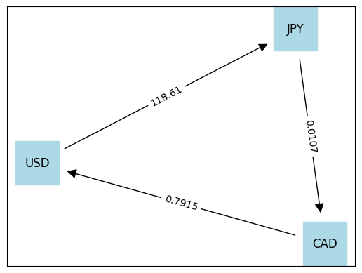
display_graph(m)
100.00000 USD -> 11861.00000 JPY -> 126.91270 CAD -> 100.45140 USD
FOREX data#
https://www.bloomberg.com/markets/currencies/cross-rates
https://www.tradingview.com/markets/currencies/cross-rates-overview-prices/
# data extracted 2022-03-17

bloomberg = """
	USD	EUR	JPY	GBP	CHF	CAD	AUD	HKD
USD	-	1.1096	0.0084	1.3148	1.0677	0.7915	0.7376	0.1279
EUR	0.9012	-	0.0076	1.1849	0.9622	0.7133	0.6647	0.1153
JPY	118.6100	131.6097	-	155.9484	126.6389	93.8816	87.4867	15.1724
GBP	0.7606	0.8439	0.0064	-	0.8121	0.6020	0.5610	0.0973
CHF	0.9366	1.0393	0.0079	1.2314	-	0.7413	0.6908	0.1198
CAD	1.2634	1.4019	0.0107	1.6611	1.3489	-	0.9319	0.1616
AUD	1.3557	1.5043	0.0114	1.7825	1.4475	1.0731	-	0.1734
HKD	7.8175	8.6743	0.0659	10.2784	8.3467	6.1877	5.7662	-
"""

df = pd.read_csv(io.StringIO(bloomberg.replace("-", "1.0")), sep="\t", index_col=0)
display(df)
| USD | EUR | JPY | GBP | CHF | CAD | AUD | HKD | |
|---|---|---|---|---|---|---|---|---|
| USD | 1.0000 | 1.1096 | 0.0084 | 1.3148 | 1.0677 | 0.7915 | 0.7376 | 0.1279 |
| EUR | 0.9012 | 1.0000 | 0.0076 | 1.1849 | 0.9622 | 0.7133 | 0.6647 | 0.1153 |
| JPY | 118.6100 | 131.6097 | 1.0000 | 155.9484 | 126.6389 | 93.8816 | 87.4867 | 15.1724 |
| GBP | 0.7606 | 0.8439 | 0.0064 | 1.0000 | 0.8121 | 0.6020 | 0.5610 | 0.0973 |
| CHF | 0.9366 | 1.0393 | 0.0079 | 1.2314 | 1.0000 | 0.7413 | 0.6908 | 0.1198 |
| CAD | 1.2634 | 1.4019 | 0.0107 | 1.6611 | 1.3489 | 1.0000 | 0.9319 | 0.1616 |
| AUD | 1.3557 | 1.5043 | 0.0114 | 1.7825 | 1.4475 | 1.0731 | 1.0000 | 0.1734 |
| HKD | 7.8175 | 8.6743 | 0.0659 | 10.2784 | 8.3467 | 6.1877 | 5.7662 | 1.0000 |
m = arbitrage(3, df, "USD")
print(f"\nInitial wealth: {m.w['USD', 0]():11.5f} USD")
print(f"Final wealth:   {m.w['USD', 3]():11.5f} USD")
Running HiGHS 1.5.3 [date: 2023-05-16, git hash: 594fa5a9d]
Copyright (c) 2023 HiGHS under MIT licence terms

t = 0

w[USD,0] =   100.00000
w[EUR,0] =     0.00000
w[JPY,0] =     0.00000
w[GBP,0] =     0.00000
w[CHF,0] =     0.00000
w[CAD,0] =     0.00000
w[AUD,0] =     0.00000
w[HKD,0] =     0.00000

t = 1

USD -> JPY  Convert   100.00000 USD to 11861.00000 JPY

w[USD,1] =     0.00000
w[EUR,1] =     0.00000
w[JPY,1] = 11861.00000
w[GBP,1] =     0.00000
w[CHF,1] =     0.00000
w[CAD,1] =     0.00000
w[AUD,1] =     0.00000
w[HKD,1] =     0.00000

t = 2

JPY -> CAD  Convert 11861.00000 JPY to   126.91270 CAD

w[USD,2] =     0.00000
w[EUR,2] =     0.00000
w[JPY,2] =     0.00000
w[GBP,2] =     0.00000
w[CHF,2] =     0.00000
w[CAD,2] =   126.91270
w[AUD,2] =     0.00000
w[HKD,2] =     0.00000

t = 3

CAD -> USD  Convert   126.91270 CAD to   100.45140 USD

w[USD,3] =   100.45140
w[EUR,3] =     0.00000
w[JPY,3] =     0.00000
w[GBP,3] =     0.00000
w[CHF,3] =     0.00000
w[CAD,3] =     0.00000
w[AUD,3] =     0.00000
w[HKD,3] =     0.00000

Initial wealth:   100.00000 USD
Final wealth:     100.45140 USD
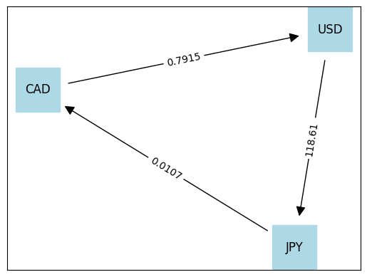
display_graph(m)
100.00000 USD -> 11861.00000 JPY -> 126.91270 CAD -> 100.45140 USD