4.5 Cryptocurrency arbitrage search

4.5 Cryptocurrency arbitrage search#

Installations and Imports#

Preamble: Install Pyomo and a solver#

The following cell sets and verifies a global SOLVER for the notebook. If run on Google Colab, the cell installs Pyomo and the HiGHS solver, while, if run elsewhere, it assumes Pyomo and HiGHS have been previously installed. It then sets to use HiGHS as solver via the appsi module and a test is performed to verify that it is available. The solver interface is stored in a global object SOLVER for later use.

import sys
 
if 'google.colab' in sys.modules:
    %pip install pyomo >/dev/null 2>/dev/null
    %pip install highspy >/dev/null 2>/dev/null
 
solver = 'appsi_highs'
 
import pyomo.environ as pyo
SOLVER = pyo.SolverFactory(solver)

assert SOLVER.available(), f"Solver {solver} is not available."

Problem description#

Cryptocurrency exchanges are web services that enable the purchase, sale, and exchange of cryptocurrencies. These exchanges provide liquidity for owners and establish the relative value of these currencies. Joining an exchange enables a user to maintain multiple currencies in a digital wallet, buy and sell currencies, and use cryptocurrencies for financial transactions.

In this notebook, we explore the efficiency of cryptocurrency exchanges by testing for arbitrage opportunities. An arbitrage exists if a customer can realize a net profit through a sequence of risk-free trades. The efficient market hypothesis assumes arbitrage opportunities are quickly identified and exploited by investors. As a result of their trading, prices reach a new equilibrium so that any arbitrage opportunities would be small and fleeting in an efficient market. The question here is whether it is possible, with real-time data and rapid execution, for a trader to profit from these fleeting arbitrage opportunities.

Additional libraries needed: NetworkX and CCXT#

This notebook uses two additional libraries: NetworkX and CCXT.

NetworkX is a Python library for the creation, manipulation, and study of the structure, dynamics, and functions of complex networks, which is installed by deafult on Google Colab.

CCXT is an open-source library for connecting to cryptocurrency exchanges. The CCXT library is not installed by default in Google Colab, so it must be installed with the following command.

%pip install ccxt

%pip install ccxt

We import all the libraries we need for this notebook in the following cell.

import numpy as np
import pandas as pd
import matplotlib.pyplot as plt
import networkx as nx
import ccxt
import glob

Available cryptocurrency exchanges#

Here we use the ccxt library and list current exchanges supported by ccxt.

print("Available exchanges:\n")
for i, exchange in enumerate(ccxt.exchanges):
    print(f"{i+1:3d}) {exchange.ljust(20)}", end="" if (i + 1) % 4 else "\n")

Available exchanges:

  1) ace                   2) alpaca                3) ascendex              4) bequant             
  5) bigone                6) binance               7) binancecoinm          8) binanceus           
  9) binanceusdm          10) bit2c                11) bitbank              12) bitbay              
 13) bitbns               14) bitcoincom           15) bitfinex             16) bitfinex2           
 17) bitflyer             18) bitforex             19) bitget               20) bithumb             
 21) bitmart              22) bitmex               23) bitopro              24) bitpanda            
 25) bitrue               26) bitso                27) bitstamp             28) bitstamp1           
 29) bittrex              30) bitvavo              31) bkex                 32) bl3p                
 33) blockchaincom        34) btcalpha             35) btcbox               36) btcmarkets          
 37) btctradeua           38) btcturk              39) bybit                40) cex                 
 41) coinbase             42) coinbaseprime        43) coinbasepro          44) coincheck           
 45) coinex               46) coinfalcon           47) coinmate             48) coinone             
 49) coinsph              50) coinspot             51) cryptocom            52) currencycom         
 53) delta                54) deribit              55) digifinex            56) exmo                
 57) fmfwio               58) gate                 59) gateio               60) gemini              
 61) hitbtc               62) hitbtc3              63) hollaex              64) huobi               
 65) huobijp              66) huobipro             67) idex                 68) independentreserve  
 69) indodax              70) kraken               71) krakenfutures        72) kucoin              
 73) kucoinfutures        74) kuna                 75) latoken              76) lbank               
 77) lbank2               78) luno                 79) lykke                80) mercado             
 81) mexc                 82) mexc3                83) ndax                 84) novadax             
 85) oceanex              86) okcoin               87) okex                 88) okex5               
 89) okx                  90) paymium              91) phemex               92) poloniex            
 93) poloniexfutures      94) probit               95) tidex                96) timex               
 97) tokocrypto           98) upbit                99) wavesexchange       100) wazirx              
101) whitebit            102) woo                 103) yobit               104) zaif                
105) zonda               

Representing an exchange as a directed graph#

First, we need some terminology. Trading between two specific currencies is called a market, with each exchange hosting multiple markets. ccxt labels each market with a symbol common across exchanges. The market symbol is an upper-case string with abbreviations for a pair of traded currencies separated by a slash (\(/\)). The first abbreviation is the base currency, the second is the quote currency. Prices for the base currency are denominated in units of the quote currency. As an example, \(ETH/BTC\) refers to a market for the base currency Ethereum (ETH) quoted in units of the Bitcoin (BTC). The same market symbol can refer to an offer to sell the base currency (a ‘bid’) or to an offer to sell the base currency (an ‘ask’). For example, \(x\) ETH/BTC means you can buy \(x\) units of BTC with one unit of ETH.

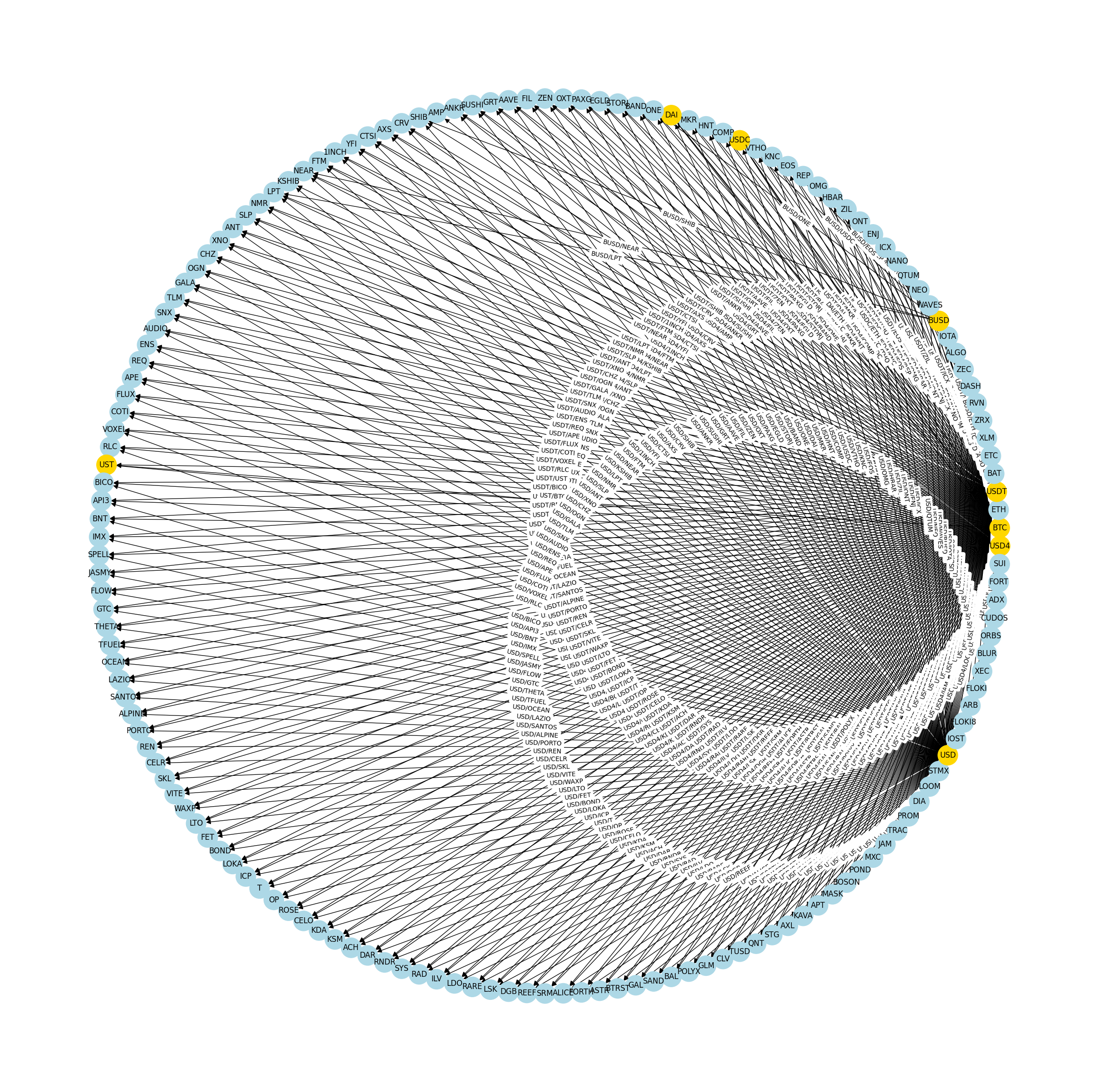
An exchange can be represented by a directed graph constructed from the market symbols available on that exchange. In such a graph currencies correspond to nodes on the directed graph. Market symbols correspond to edges in the directed graph, with the source indicating the quote currency and the destination indicating the base currency. The following code develops such a sample graph.

# create an exchange object
exchange = ccxt.binanceus()


def get_exchange_dg(exchange, minimum_in_degree=1):
    markets = exchange.load_markets()
    symbols = markets.keys()

    # create an edge for all market symbols
    dg = nx.DiGraph()
    for base, quote in [symbol.split("/") for symbol in symbols]:
        dg.add_edge(quote, base, color="k", width=1)

    # remove base currencies with in_degree less than minimum_in_degree
    remove_nodes = [
        node
        for node in dg.nodes
        if dg.out_degree(node) == 0 and dg.in_degree(node) < minimum_in_degree
    ]
    for node in reversed(list(nx.topological_sort(dg))):
        if node in remove_nodes:
            dg.remove_node(node)
        else:
            break

    # color quote currencies in gold
    for node in dg.nodes():
        dg.nodes[node]["color"] = "gold" if dg.out_degree(node) > 0 else "lightblue"

    return dg


def draw_dg(dg, rad=0.0):
    n_nodes = len(dg.nodes)
    size = int(2.5 * np.sqrt(n_nodes))
    fig = plt.figure(figsize=(size, size))
    pos = nx.circular_layout(dg)
    nx.draw_networkx(
        dg,
        pos,
        with_labels=True,
        node_color=[dg.nodes[node]["color"] for node in dg.nodes()],
        edge_color=[dg.edges[u, v]["color"] for u, v in dg.edges],
        width=[dg.edges[u, v]["width"] for u, v in dg.edges],
        node_size=1000,
        font_size=12,
        arrowsize=15,
        connectionstyle=f"arc3, rad={rad}",
    )
    nx.draw_networkx_edge_labels(
        dg, pos, edge_labels={(src, dst): f"{src}/{dst}" for src, dst in dg.edges()}
    )
    plt.axis("off")

    return plt.gca()


minimum_in_degree = 10
exchange_dg = get_exchange_dg(exchange, minimum_in_degree)
ax = draw_dg(exchange_dg, 0.01)
print(
    exchange.name
    + f" - Network obtained filtering for minimum indegree (Base Currencies) = {minimum_in_degree}"
)
print(f"Number of nodes = {len(exchange_dg.nodes()):3d}")
print(f"Number of edges = {len(exchange_dg.edges()):3d}")

Binance US - Network obtained filtering for minimum indegree (Base Currencies) = 10
Number of nodes = 155
Number of edges = 449

../../_images/331e0c01101d7ba15285fdc6bd15ab5c93717fb08397a2be205230b90d946bb0.png

Exchange order book#

The order book for a currency exchange is the real-time inventory of trading orders.

A bid is an offer to buy up to a specified amount of the base currency at the price not exceeding the ‘bid price’ in the quote currency. An ask is an offer to sell up to a specified amount of the base currency at a price no less than a value specified given in the quote currency.

The exchange attempts to match the bid to ask order at a price less than or equal to the bid price. If a transaction occurs, the buyer will receive an amount of base currency less than or equal to the bid volume and the ask volume, at a price less than or equal to the bid price and no less than the specified value.

The order book for currency exchange is the real-time inventory of orders. The exchange order book maintains a list of all active orders for symbols traded on the exchange. Incoming bids above the lowest ask or incoming asks below the highest bid will be immediately matched and transactions executed following the rules of the exchange.

The following cell reads and displays a previously saved order book. Cells at the end of this notebook demonstrate how to retrieve an order book from an exchange and save it as a Pandas DataFrame.

filename = "Binance_US_orderbook_saved.csv"
if "google.colab" in sys.modules:
    order_book = pd.read_csv(
        "https://raw.githubusercontent.com/mobook/MO-book/main/notebooks/04/data/"
        + filename,
        index_col=0,
    )
else:
    order_book = pd.read_csv("data/" + filename, index_col=0)

display(order_book)

	symbol	timestamp	base	quote	bid_price	bid_volume	ask_price	ask_volume
0	ETH/BTC	2023-03-02 15:36:06.529	ETH	BTC	0.069735	0.012000	0.069759	0.050000
1	BNB/BTC	2023-03-02 15:36:06.583	BNB	BTC	0.012743	0.050000	0.012755	3.000000
2	ADA/BTC	2023-03-02 15:36:06.637	ADA	BTC	0.000015	2.000000	0.000015	2168.000000
3	SOL/BTC	2023-03-02 15:36:06.690	SOL	BTC	0.000935	1.420000	0.000936	15.120000
4	MATIC/BTC	2023-03-02 15:36:06.750	MATIC	BTC	0.000052	26.200000	0.000052	150.200000
5	MANA/BTC	2023-03-02 15:36:06.848	MANA	BTC	0.000027	831.000000	0.000027	1409.000000
6	TRX/BTC	2023-03-02 15:36:06.905	TRX	BTC	0.000003	4.000000	0.000003	25352.000000
7	ADA/ETH	2023-03-02 15:36:06.960	ADA	ETH	0.000214	994.900000	0.000214	891.600000
8	BTC/USDT	2023-03-02 15:36:07.012	BTC	USDT	23373.920000	0.118619	23376.000000	0.045275
9	ETH/USDT	2023-03-02 15:36:07.065	ETH	USDT	1630.200000	0.950000	1630.770000	0.500000
10	BNB/USDT	2023-03-02 15:36:07.118	BNB	USDT	297.857700	0.800000	297.891900	0.800000
11	ADA/USDT	2023-03-02 15:36:07.172	ADA	USDT	0.348630	1100.000000	0.348750	511.200000
12	BUSD/USDT	2023-03-02 15:36:07.226	BUSD	USDT	0.999500	293433.930000	0.999600	317175.730000
13	SOL/USDT	2023-03-02 15:36:07.288	SOL	USDT	21.857000	22.870000	21.863500	23.000000
14	USDC/USDT	2023-03-02 15:36:07.342	USDC	USDT	1.000100	307657.000000	1.000200	299181.000000
15	MATIC/USDT	2023-03-02 15:36:07.394	MATIC	USDT	1.203000	1664.600000	1.205000	5405.600000
16	MANA/USDT	2023-03-02 15:36:07.447	MANA	USDT	0.631000	157.000000	0.632200	571.000000
17	TRX/USDT	2023-03-02 15:36:07.501	TRX	USDT	0.069280	10824.900000	0.069330	10818.600000
18	BTC/BUSD	2023-03-02 15:36:07.612	BTC	BUSD	23371.440000	0.021500	23376.830000	0.021500
19	BNB/BUSD	2023-03-02 15:36:07.665	BNB	BUSD	297.763000	1.670000	297.952500	1.340000
20	ETH/BUSD	2023-03-02 15:36:07.719	ETH	BUSD	1630.210000	0.510000	1630.760000	0.255000
21	MATIC/BUSD	2023-03-02 15:36:07.772	MATIC	BUSD	1.203410	623.100000	1.204540	415.000000
22	USDC/BUSD	2023-03-02 15:36:07.893	USDC	BUSD	0.999900	329027.800000	1.000000	279879.620000
23	MANA/BUSD	2023-03-02 15:36:07.950	MANA	BUSD	0.630700	343.000000	0.632100	3054.000000
24	ADA/BUSD	2023-03-02 15:36:08.003	ADA	BUSD	0.348000	6582.900000	0.349000	997.000000
25	SOL/BUSD	2023-03-02 15:36:08.056	SOL	BUSD	21.830000	1.390000	21.900000	181.090000
26	TRX/BUSD	2023-03-02 15:36:08.114	TRX	BUSD	0.069290	10823.900000	0.069390	25220.400000
27	BTC/USDC	2023-03-02 15:36:08.170	BTC	USDC	23371.660000	0.020000	23376.990000	0.051000
28	ETH/USDC	2023-03-02 15:36:08.228	ETH	USDC	1630.160000	0.100000	1630.810000	0.215000
29	SOL/USDC	2023-03-02 15:36:08.298	SOL	USDC	21.830000	343.520000	21.880000	201.080000
30	ADA/USDC	2023-03-02 15:36:08.368	ADA	USDC	0.348200	8615.400000	0.349400	2433.100000
31	BTC/DAI	2023-03-02 15:36:08.433	BTC	DAI	23366.440000	0.049540	23394.360000	0.049500
32	ETH/DAI	2023-03-02 15:36:08.485	ETH	DAI	1629.890000	0.497400	1631.810000	1.490000
33	BTC/USD	2023-03-02 15:36:08.623	BTC	USD	23373.010000	0.007463	23376.720000	0.048805
34	ETH/USD	2023-03-02 15:36:08.675	ETH	USD	1630.490000	2.564550	1630.740000	0.580700
35	USDT/USD	2023-03-02 15:36:08.730	USDT	USD	1.000000	10407.870000	1.000100	954839.680000
36	BNB/USD	2023-03-02 15:36:08.782	BNB	USD	297.900200	2.100000	297.952500	1.342000
37	ADA/USD	2023-03-02 15:36:08.835	ADA	USD	0.348800	1500.000000	0.348900	3000.000000
38	BUSD/USD	2023-03-02 15:36:08.942	BUSD	USD	0.999500	79157.800000	0.999900	795593.480000
39	MATIC/USD	2023-03-02 15:36:08.998	MATIC	USD	1.204000	937.600000	1.204500	937.500000
40	USDC/USD	2023-03-02 15:36:09.051	USDC	USD	0.999900	5050.300000	1.000000	517682.170000
41	MANA/USD	2023-03-02 15:36:09.102	MANA	USD	0.631000	372.340000	0.631600	572.340000
42	DAI/USD	2023-03-02 15:36:09.155	DAI	USD	0.999100	4534.660000	1.000100	7591.820000
43	SOL/USD	2023-03-02 15:36:09.217	SOL	USD	21.858100	55.730000	21.865900	18.290000
44	TRX/USD	2023-03-02 15:36:09.270	TRX	USD	0.069200	225602.200000	0.069400	224245.500000

Modelling the arbitrage search problem as a graph#

Our goal will be to find arbitrage opportunities, i.e., the possibility to start from a given currency and, through a sequence of executed trades, arrive back at the same currency with a higher balance than at the beginning. We will model this problem as a network one.

A bid appearing in the order book for the market symbol \(b/q\) is an order from a prospective counter party to purchase an amount of the base currency \(b\) at a bid price given in a quote currency \(q\). For a currency trader, a bid in the order book is an opportunity to convert the base currency \(b\) into the quote currency \(q\).

The order book can be represented as a directed graph where the nodes correspond to individual currencies. A directed edge \(b\rightarrow q\) from node \(b\) to node \(q\) describes an opportunity for us to convert currency \(b\) into units of currency \(q\). Let \(V_b\) and \(V_q\) denote the amounts of each currency held by us, and let \(x_{b\rightarrow q}\) denote the amount of currency \(b\) exchanged for currency \(j\). Following the transaction \(x_{b\rightarrow q}\) we have the following changes to the currency holdings

\[\begin{split} \begin{align*} \Delta V_b & = - x_{b\rightarrow q} \\ \Delta V_q & = a_{b\rightarrow q} x_{b\rightarrow q}, \end{align*} \end{split}\]

where \(a_{b\rightarrow q}\) is a conversion coefficient equal to the price of \(b\) expressed in terms of currency \(q\). The capacity \(c_{b\rightarrow q}\) of a trading along edge \(b\rightarrow q\) is specified by a relationship

\[ x_{b\rightarrow q} \leq c_{b\rightarrow q}. \]

Because the arcs in our graph correspond to two types of orders - bid and ask - we need to build a consistent way of expressing them in our \(a_{b\rightarrow q}\), \(c_{b\rightarrow q}\) notation. Imagine now that we are the party that accepts the buy and ask bids existing in the graph.

For bid orders, we have the opportunity to convert the base currency \(b\) into the quote currency \(q\), for which we will use the following notation:

\[\begin{split} \begin{align*} a_{b\rightarrow q} & = \text{bid price} \\ c_{b\rightarrow q} & = \text{bid volume} \end{align*} \end{split}\]

An ask order for symbol \(b/q\) is an order to sell the base currency at a price not less than the ‘ask’ price given in terms of the quote currency. The ask volume is the amount of base currency to be sold. For us, a sell order is an opportunity to convert the quoted currency into the base currency such that

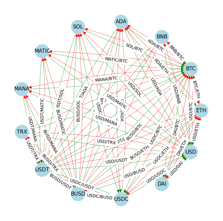
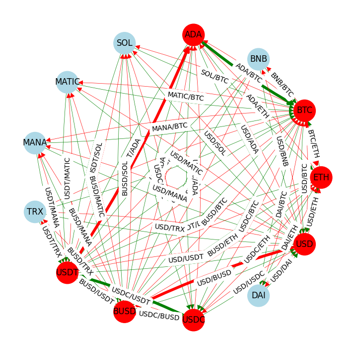
\[\begin{split} \begin{align*} a_{q\rightarrow b} & = \frac{1}{\text{ask price}} \\ c_{q\rightarrow b} & = \text{ask volume} \times \text{ask volume} \end{align*} \end{split}\]

The following cell creates a directed graph using data from an exchange order book. To distinguish between different order types, we will highlight the big orders with green color, and ask orders with red color.

def order_book_to_dg(order_book):
    # create a dictionary of edges index by (src, dst)
    dg_order_book = nx.DiGraph()

    # loop over each order in the order book dataframe
    for order in order_book.index:
        # if the order is a 'bid', i.e., an order to purchase the base currency
        if not np.isnan(order_book.at[order, "bid_volume"]):
            src = order_book.at[order, "base"]
            dst = order_book.at[order, "quote"]
            # add an edge to the graph with the relevant attributes
            dg_order_book.add_edge(
                src,
                dst,
                kind="bid",
                a=order_book.at[order, "bid_price"],
                capacity=order_book.at[order, "bid_volume"],
                weight=-np.log(order_book.at[order, "bid_price"]),
                color="g",
                width=0.5,
            )

        # if the order is an 'ask', i.e., an order to sell the base currency
        if not np.isnan(order_book.at[order, "ask_volume"]):
            src = order_book.at[order, "quote"]
            dst = order_book.at[order, "base"]
            # add an edge to the graph with the relevant attributes
            dg_order_book.add_edge(
                src,
                dst,
                kind="ask",
                a=1.0 / order_book.at[order, "ask_price"],
                capacity=order_book.at[order, "ask_volume"]
                * order_book.at[order, "ask_price"],
                weight=-np.log(1.0 / order_book.at[order, "ask_price"]),
                color="r",
                width=0.5,
            )

    # loop over each node in the graph and set the color attribute to "lightblue"
    for node in dg_order_book.nodes():
        dg_order_book.nodes[node]["color"] = "lightblue"

    return dg_order_book


order_book_dg = order_book_to_dg(order_book)

First, we simply print the content of the order book as a list of arcs.

# display contents of the directed graph
print(f"src   --> dst    kind            a                c")
print(f"------------------------------------------------------")
for src, dst in order_book_dg.edges():
    print(
        f"{src:5s} --> {dst:5s}   {order_book_dg.edges[(src, dst)]['kind']}"
        + f"{order_book_dg.edges[(src, dst)]['a']: 16f} {order_book_dg.edges[(src, dst)]['capacity']: 16f}    "
    )

src   --> dst    kind            a                c
------------------------------------------------------
ETH   --> BTC     bid        0.069735         0.012000    
ETH   --> ADA     ask     4668.534080         0.190981    
ETH   --> USDT    bid     1630.200000         0.950000    
ETH   --> BUSD    bid     1630.210000         0.510000    
ETH   --> USDC    bid     1630.160000         0.100000    
ETH   --> DAI     bid     1629.890000         0.497400    
ETH   --> USD     bid     1630.490000         2.564550    
BTC   --> ETH     ask       14.335068         0.003488    
BTC   --> BNB     ask       78.403701         0.038263    
BTC   --> ADA     ask    66844.919786         0.032433    
BTC   --> SOL     ask     1068.261938         0.014154    
BTC   --> MATIC   ask    19391.118868         0.007746    
BTC   --> MANA    ask    36968.576710         0.038113    
BTC   --> TRX     ask   335570.469799         0.075549    
BTC   --> USDT    bid    23373.920000         0.118619    
BTC   --> BUSD    bid    23371.440000         0.021500    
BTC   --> USDC    bid    23371.660000         0.020000    
BTC   --> DAI     bid    23366.440000         0.049540    
BTC   --> USD     bid    23373.010000         0.007463    
BNB   --> BTC     bid        0.012743         0.050000    
BNB   --> USDT    bid      297.857700         0.800000    
BNB   --> BUSD    bid      297.763000         1.670000    
BNB   --> USD     bid      297.900200         2.100000    
ADA   --> BTC     bid        0.000015         2.000000    
ADA   --> ETH     bid        0.000214       994.900000    
ADA   --> USDT    bid        0.348630      1100.000000    
ADA   --> BUSD    bid        0.348000      6582.900000    
ADA   --> USDC    bid        0.348200      8615.400000    
ADA   --> USD     bid        0.348800      1500.000000    
SOL   --> BTC     bid        0.000935         1.420000    
SOL   --> USDT    bid       21.857000        22.870000    
SOL   --> BUSD    bid       21.830000         1.390000    
SOL   --> USDC    bid       21.830000       343.520000    
SOL   --> USD     bid       21.858100        55.730000    
MATIC --> BTC     bid        0.000052        26.200000    
MATIC --> USDT    bid        1.203000      1664.600000    
MATIC --> BUSD    bid        1.203410       623.100000    
MATIC --> USD     bid        1.204000       937.600000    
MANA  --> BTC     bid        0.000027       831.000000    
MANA  --> USDT    bid        0.631000       157.000000    
MANA  --> BUSD    bid        0.630700       343.000000    
MANA  --> USD     bid        0.631000       372.340000    
TRX   --> BTC     bid        0.000003         4.000000    
TRX   --> USDT    bid        0.069280     10824.900000    
TRX   --> BUSD    bid        0.069290     10823.900000    
TRX   --> USD     bid        0.069200    225602.200000    
USDT  --> BTC     ask        0.000043      1058.348400    
USDT  --> ETH     ask        0.000613       815.385000    
USDT  --> BNB     ask        0.003357       238.313520    
USDT  --> ADA     ask        2.867384       178.281000    
USDT  --> BUSD    ask        1.000400    317048.859708    
USDT  --> SOL     ask        0.045738       502.860500    
USDT  --> USDC    ask        0.999800    299240.836200    
USDT  --> MATIC   ask        0.829876      6513.748000    
USDT  --> MANA    ask        1.581778       360.986200    
USDT  --> TRX     ask       14.423770       750.053538    
USDT  --> USD     bid        1.000000     10407.870000    
BUSD  --> USDT    bid        0.999500    293433.930000    
BUSD  --> BTC     ask        0.000043       502.601845    
BUSD  --> BNB     ask        0.003356       399.256350    
BUSD  --> ETH     ask        0.000613       415.843800    
BUSD  --> MATIC   ask        0.830192       499.884100    
BUSD  --> USDC    ask        1.000000    279879.620000    
BUSD  --> MANA    ask        1.582028      1930.433400    
BUSD  --> ADA     ask        2.865330       347.953000    
BUSD  --> SOL     ask        0.045662      3965.871000    
BUSD  --> TRX     ask       14.411298      1750.043556    
BUSD  --> USD     bid        0.999500     79157.800000    
USDC  --> USDT    bid        1.000100    307657.000000    
USDC  --> BUSD    bid        0.999900    329027.800000    
USDC  --> BTC     ask        0.000043      1192.226490    
USDC  --> ETH     ask        0.000613       350.624150    
USDC  --> SOL     ask        0.045704      4399.630400    
USDC  --> ADA     ask        2.862049       850.125140    
USDC  --> USD     bid        0.999900      5050.300000    
DAI   --> BTC     ask        0.000043      1158.020820    
DAI   --> ETH     ask        0.000613      2431.396900    
DAI   --> USD     bid        0.999100      4534.660000    
USD   --> BTC     ask        0.000043      1140.900820    
USD   --> ETH     ask        0.000613       946.970718    
USD   --> USDT    ask        0.999900    954935.163968    
USD   --> BNB     ask        0.003356       399.852255    
USD   --> ADA     ask        2.866151      1046.700000    
USD   --> BUSD    ask        1.000100    795513.920652    
USD   --> MATIC   ask        0.830220      1129.218750    
USD   --> USDC    ask        1.000000    517682.170000    
USD   --> MANA    ask        1.583281       361.489944    
USD   --> DAI     ask        0.999900      7592.579182    
USD   --> SOL     ask        0.045733       399.927311    
USD   --> TRX     ask       14.409222     15562.637700    

Next, we draw the graph itself.

draw_dg(order_book_dg, 0.05)
plt.show()

../../_images/d1d412c48358ebfbd002a217e8b904cf374f5cb716d5469a3933d357d6f8f79d.png

Trading and arbitrage#

With this unified treatment of bid and ask orders, we are ready to formulate the mathematical problem of finding an arbitrage opportunity. An arbitrage exists if it is possible to find a closed path and a sequence of transactions in the directed graph resulting in a net increase in currency holdings. Given a path

\[ \begin{align*} i_0 \rightarrow i_1 \rightarrow i_2 \rightarrow \cdots \rightarrow i_{n-1} \rightarrow i_n \end{align*} \]

the path is closed if \(i_n = i_0\). The path has finite capacity if each edge in the path has a non-zero capacity. For a sufficiently small holding \(w_{i_0}\) of currency \(i_0\) (because of capacity constraints), a closed path with \(i_0 = i_n\) represents an arbitrage opportunity if

\[ \begin{equation} \prod_{k=0}^{n-1} a_{i_k\rightarrow i_{k+1}} > 1. \end{equation} \]

If all we care about is simply finding an arbitrage cycle, regardless of the volume traded, we can use one of the many shortest path algorithms from the networkx library. To convert the problem of finding a path meeting the above condition into a sum-of-terms to be minimized, we can take the negative logarithm of both sides to obtain the condition:

\[ \begin{align*} -\log(\prod_{k=0}^{n-1} a_{i_k\rightarrow i_{k+1}}) = - \sum\limits_{k = 0}^{n-1} \log (a_{i_k\rightarrow i_{k+1}}) < 0, \end{align*} \]

In other words, if we assign the negative logarithm as the weight of arcs in a graph, then our problem just becomes translated into the problem of searching for a cycle with a total sum of weights along it to be negative.

Find order books that have arbitrage opportunities#

A simple cycle is a closed path in which no node appears twice. Simple cycles are distinct if they are not cyclic permutations (essentially, the same set of nodes but with a different start and end points) of each other. One could check for arbitrage opportunities by checking if there are any negative simple cycles in the graph.

However, searching for a negative-weight cycle through searching for an arbitrage opportunity can be a daunting task - a brute-force search over all simple cycles has complexity \((n + e)(c + 1)\) which is impractical for large-scale applications. A more efficient search based on the Bellman-Ford algorithm is embedded in the NetworkX function negative_edge_cycle that returns a logical True if a negative cycle exists in a directed graph.

order_book_dg = order_book_to_dg(order_book)
nx.negative_edge_cycle(order_book_dg, weight="weight", heuristic=True)

True

The function negative_edge_cycle is fast, but it only indicates if there is a negative cycle or not, and we don’t even know what kind of a cycle is it so it would be hard to use that information to perform an arbitrage.

Luckily, the networkx library includes the function find_negative_cycle that locates a single negative edge cycle if one exists. We can use this to demonstrate the existence of an arbitrage opportunity and to highlight that opportunity on the directed graph of all possible trades. The following cell reports the cycle found and the corresponding trading return measured in basis points (1 basis point = 0.01%). The same trading cycle is marked with thicker arcs in the graph.

def sum_weights(cycle):
    return sum(
        [
            order_book_dg.edges[edge]["weight"]
            for edge in zip(cycle, cycle[1:] + cycle[:1])
        ]
    )


order_book_dg = order_book_to_dg(order_book)
arb = nx.find_negative_cycle(order_book_dg, weight="weight", source="USD")[:-1]
bp = 10000 * (np.exp(-sum_weights(arb)) - 1)

for src, dst in zip(arb, arb[1:] + arb[:1]):
    order_book_dg[src][dst]["width"] = 5

print(
    f"Trading cycle with {len(list(arb))} trades: {' --> '.join(list(arb))}\nReturn = {bp:6.3f} basis points "
)
ax = draw_dg(order_book_dg, 0.05)
plt.show()

Trading cycle with 3 trades: USDC --> USDT --> BUSD
Return =  5.002 basis points 

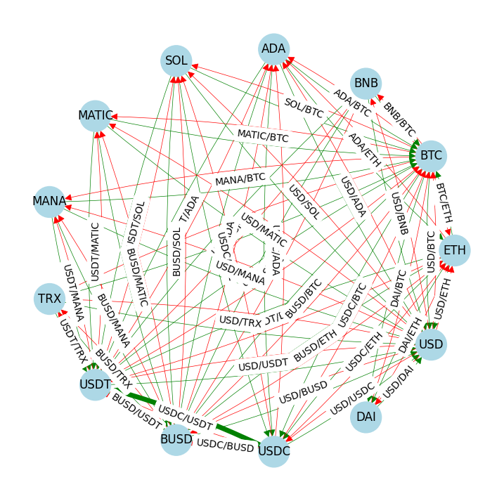
../../_images/b7839168395c04636d4d3ca4880e56ce3ffe27de0cd4c53c54a3e897603f126e.png

Note this may or may not be the trading cycle with maximum return. There may be other cycles with higher or lower returns, and that allow higher or lower trading volumes.

Brute force search arbitrage with simple cycles#

Not all arbitrage cycles are the same - some yield a higher relative return (per dollar invested) than the others, and some yield a higher absolute return (maximum amount of money to be made risk-free) than others. This is because the amount of money that flows through a negative cycle is upper bounded by the size of the smallest order in that cycle. Thus, if one is looking for the best possible arbitrage sequence of trades, finding just ‘a cycle’ might not be enough.

A crude way to search for a good arbitrage opportunity would be to enumerate all possible simple cycles in a graph and pick the one that’s best according to whatever criterion we pick. A brute force search over for all simple cycles has order \((N_{nodes} + N_{edges})(N_{cycles} + 1)\) complexity, which is prohibitive for large order books. Nevertheless, we explore this option here to better understand the problem of finding and valuing arbitrage opportunities.

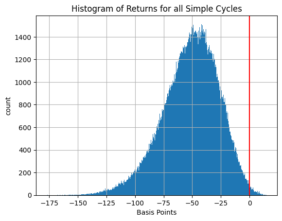
In the following cell, we compute the loss function for all simple cycles that can be constructed within a directed graph using the function simple_cycles from the networkx library to construct a dictionary of all distinct simple cycles in the order book. Each cycle is represented by an ordered list of nodes. For each cycle, the financial return is computed, and a histogram is constructed to show the distribution of potential returns. Several paths with the highest return are then overlaid on the graph of the order book.

Again, note that no account is taken of the trading capacity available on each path.

The next cell iterates over all simple cycles in a directed graph. This can take a long time for a large dense graph.

# convert order book to a directed graph
order_book_dg = order_book_to_dg(order_book)


# compute the sum of weights given a list of nodes
def sum_weights(cycle):
    return sum(
        [
            order_book_dg.edges[edge]["weight"]
            for edge in zip(cycle, cycle[1:] + cycle[:1])
        ]
    )


# create a dictionary of all simple cycles and sum of weights
cycles = {
    tuple(cycle): 10000 * (np.exp(-sum_weights(cycle)) - 1)
    for cycle in nx.simple_cycles(order_book_dg)
}

print(
    f"There are {len(cycles)} distinct simple cycles in the order book, {len([cycle for cycle in cycles if cycles[cycle] > 0])} of which have positive return."
)

# create histogram
plt.hist(cycles.values(), bins=int(np.sqrt(len(cycles))))
ax = plt.gca()
ax.set_ylabel("count")
ax.set_xlabel("Basis Points")
ax.set_title("Histogram of Returns for all Simple Cycles")
ax.grid(True)
ax.axvline(0, color="r")
plt.show()

There are 203147 distinct simple cycles in the order book, 974 of which have positive return.

../../_images/84ebc76f8acac6bb9ebd870a9eb7f70e1db739c2d6bd2d3bf50f5f056e2f8429.png

Next, we sort out the negative cycles from this list and present them along with their basis-points (1% is 100 basis points) return.

arbitrage = [
    cycle for cycle in sorted(cycles, key=cycles.get, reverse=True) if cycles[cycle] > 0
]

n_cycles_to_list = 5

print(f"Top {n_cycles_to_list}\n")
print(f"Basis Points             Arbitrage Cycle")
for cycle in arbitrage[0 : min(n_cycles_to_list, len(arbitrage))]:
    t = list(cycle)
    t.append(cycle[0])
    print(f"{cycles[cycle]:6.3f}         {len(t)} trades: {' --> '.join(t)}")

Top 5

Basis Points             Arbitrage Cycle
774         8 trades: USDT --> ADA --> BTC --> ETH --> USD --> BUSD --> USDC --> USDT
747         8 trades: USDT --> TRX --> BTC --> ETH --> USD --> BUSD --> USDC --> USDT
699         7 trades: USDT --> ADA --> BTC --> USD --> BUSD --> USDC --> USDT
673         7 trades: USDT --> TRX --> BTC --> USD --> BUSD --> USDC --> USDT
772         7 trades: USDT --> ADA --> BTC --> ETH --> USD --> USDC --> USDT

In the end, we draw an example arbitrage cycle on our graph to illustrate the route that the money must travel.

n_cycles_to_show = 1

for cycle in arbitrage[0 : min(n_cycles_to_show, len(arbitrage))]:
    print(
        f"Trading cycle with {len(t)} trades: {' --> '.join(t)}\nReturn = {cycles[cycle]:6.3f} basis points "
    )
    # get fresh graph to color nodes
    order_book_dg = order_book_to_dg(order_book)

    # color nodes red
    for node in cycle:
        order_book_dg.nodes[node]["color"] = "red"

    # makes lines wide
    for edge in zip(cycle, cycle[1:] + cycle[:1]):
        order_book_dg.edges[edge]["width"] = 4

    ax = draw_dg(order_book_dg, rad=0.05)

    t = list(cycle)
    t.append(cycle[0])
    plt.show()

Trading cycle with 8 trades: USDT --> ADA --> BTC --> ETH --> USD --> BUSD --> USDC --> USDT
Return = 14.774 basis points 

../../_images/c3018b18d57bdbfb0d81a1d2b0865cddf1fbdc3546ef55dd637ea008e8ec1e65.png

Pyomo model for arbitrage with capacity constraints#

The preceding analysis demonstrates some practical limitations of relying on generic implementations of network algorithms:

First, more than one negative cycle may exist, so more than one arbitrage opportunity may exist, i.e. an optimal strategy consists of a combination of cycles.
Secondly, simply searching for a negative cycle using shortest path algorithms does not account for capacity constraints, i.e., the maximum size of each of the exchanges. For that reason, one may end up with a cycle on which a good `rate’ of arbitrage is available, but where the absolute gain need not be large due to the maximum amounts that can be traded.

Instead, we can formulate the problem of searching for a maximum-gain arbitrage via linear optimization. Assume that we are given a directed graph where each edge \(i\rightarrow j\) is labeled with a ‘multiplier’ \(a_{i\rightarrow j}\) indicating how many units of currency \(j\) will be received for one unit of currency \(i\), and a ‘capacity’ \(c_{i\rightarrow j}\) indicating how many units of currency \(i\) can be converted to currency \(j\).

We break the trading process into steps indexed by \(t = 1, 2, \ldots, T\), where currencies are exchanged between two adjacent nodes in a single step. We denote by \(x_{i\rightarrow j}(t)\) the amount of currency traded from node \(i\) to \(j\) in step \(t\). In this way, we start with the amount \(w_{USD}(0)\) at time \(0\) and aim to maximize the amount \(w_{USD}(T)\) at time \(T\). Denote by \(O_j\) the set of nodes to which outgoing arcs from \(j\) lead, and by \(I_j\) the set of nodes from which incoming arcs lead.

A single transaction converts \(x_{i\rightarrow j}(t)\) units of currency \(i\) to currency \(j\). Following all transactions at event \(t\), the trader will hold \(v_j(t)\) units of currency \(j\) where

\[v_{j}(t) = v_{j}(t-1) + \sum_{i\in I_j} a_{i\rightarrow j}x_{i\rightarrow j}(t) - \sum_{k\in O_j} x_{j\rightarrow k}(t)\]

For every edge \(i\rightarrow j\), the sum of all transactions must satisfy

\[\sum_{t=1}^T x_{j\rightarrow k}(t) \leq c_{j\rightarrow k}\]

The objective of the optimization model is to find a sequence of currency transactions that increase the holdings of a reference currency. The solution is constrained by assuming that the trader cannot short sell any currency. The resulting model is

\[\begin{split} \begin{align*} \max \quad & v_{USD}(T) \\ \text{s.t.} \quad & v_{USD}(0) = v_0 \\ & v_{j}(t) = v_{j}(t-1) + \sum_{i\in I_j} a_{i\rightarrow j}x_{i\rightarrow j}(t) - \sum_{k\in O_j} x_{j\rightarrow k}(t) & \forall j\in N, t=1, 2, \ldots, T \\ & v_j(t-1) \geq \sum_{k\in O_j} x_{j\rightarrow k}(t) & \forall j\in N, t = 1, 2, \ldots, T \\ & \sum_{t=1}^T x_{j\rightarrow k}(t) \leq c_{j\rightarrow k} & \forall (j, k) \in E, t = 1, 2, \ldots, T \\ & v_{j}(t), x_{i\rightarrow j}(t) \geq 0 & \forall t \end{align*} \end{split}\]

where the constraints model:

the initial amount condition,
the balance equations linking the state of the given node in the previous and subsequent time periods,
the fact that we cannot trade at time step \(t\) more of a given currency than we had in this currency from time step \(t - 1\). This constraint ‘enforces’ the time order of trades, i.e., we cannot trade in time period \(t\) units which have been received in the same time period.
the maximum allowed trade volumes,
the non-negativity of the variables.

The following cell implements this optimization model using Pyomo.

def crypto_model(order_book_dg, T=10, v0=100.0):
    m = pyo.ConcreteModel("Cryptocurrency arbitrage")

    # length of the trading chain
    m.T0 = pyo.RangeSet(0, T)
    m.T1 = pyo.RangeSet(1, T)

    # currency nodes and trading edges
    m.NODES = pyo.Set(initialize=list(order_book_dg.nodes))
    m.EDGES = pyo.Set(initialize=list(order_book_dg.edges))

    # currency on hand at each node
    m.v = pyo.Var(m.NODES, m.T0, domain=pyo.NonNegativeReals)

    # amount traded on each edge at each trade
    m.x = pyo.Var(m.EDGES, m.T1, domain=pyo.NonNegativeReals)

    # total amount traded on each edge over all trades
    m.z = pyo.Var(m.EDGES, domain=pyo.NonNegativeReals)

    # "multiplier" on each trading edge
    @m.Param(m.EDGES)
    def a(m, src, dst):
        return order_book_dg.edges[(src, dst)]["a"]

    @m.Param(m.EDGES)
    def c(m, src, dst):
        return order_book_dg.edges[(src, dst)]["capacity"]

    @m.Objective(sense=pyo.maximize)
    def wealth(m):
        return m.v["USD", T]

    @m.Constraint(m.EDGES)
    def total_traded(m, src, dst):
        return m.z[src, dst] == sum([m.x[src, dst, t] for t in m.T1])

    @m.Constraint(m.EDGES)
    def edge_capacity(m, src, dst):
        return m.z[src, dst] <= m.c[src, dst]

    # initial assignment of v0 units on a selected currency
    @m.Constraint(m.NODES)
    def initial(m, node):
        if node == "USD":
            return m.v[node, 0] == v0
        return m.v[node, 0] == 0

    @m.Constraint(m.NODES, m.T1)
    def no_shorting(m, node, t):
        out_nodes = [dst for src, dst in m.EDGES if src == node]
        return m.v[node, t - 1] >= sum(m.x[node, dst, t] for dst in out_nodes)

    @m.Constraint(m.NODES, m.T1)
    def balances(m, node, t):
        in_nodes = [src for src, dst in m.EDGES if dst == node]
        out_nodes = [dst for src, dst in m.EDGES if src == node]
        return m.v[node, t] == m.v[node, t - 1] + sum(
            m.a[src, node] * m.x[src, node, t] for src in in_nodes
        ) - sum(m.x[node, dst, t] for dst in out_nodes)

    return m

Using this function, we are able to compute the optimal (absolute) return from an order book while respecting the order capacities and optimally using all the arbitrage opportunities inside it.

order_book_dg = order_book_to_dg(order_book)
v0 = 10000.0
T = 8
m = crypto_model(order_book_dg, T=T, v0=v0)
SOLVER.solve(m)
vT = m.wealth()

print(f"Starting wealth = {v0:0.2f} USD")
print(f"Weath after {T:2d} transactions = {vT:0.2f} USD")
print(f"Return = {10000 * (vT - v0)/v0:0.3f} basis points")

Starting wealth = 10000.00 USD
Weath after  8 transactions = 10009.01 USD
Return = 9.006 basis points

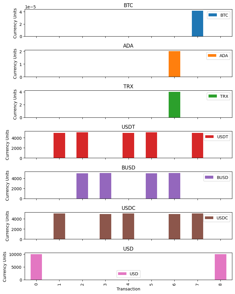
To track the evolution of the trades throughout time, the script in the following cell illustrates, for each currency (rows) the amount of money held in that currency at each of the time steps \(t = 0, \dots, 8\). It is visible from this scheme that the sequence of trades is not a simple cycle, but rather a more sophisticated sequence of trades which we would not have discovered with simple-cycle exploration alone, especially not when considering also the arc capacities.

for node in m.NODES:
    print(f"{node:5s}", end="")
    for t in m.T0:
        print(f" {m.v[node, t]():11.5f}", end="")
    print()

ETH       0.00000     0.00000     0.00000     0.00000     0.00000     0.00000     0.00000     0.00000     0.00000
BTC       0.00000     0.00000     0.00000     0.00000     0.00000     0.00000     0.00000     0.00004     0.00000
BNB       0.00000     0.00000     0.00000     0.00000     0.00000     0.00000     0.00000     0.00000     0.00000
ADA       0.00000     0.00000     0.00000     0.00000     0.00000     0.00000     2.00000     0.00000     0.00000
SOL       0.00000     0.00000     0.00000     0.00000     0.00000     0.00000     0.00000     0.00000     0.00000
MATIC     0.00000     0.00000     0.00000     0.00000     0.00000     0.00000     0.00000     0.00000     0.00000
MANA      0.00000     0.00000     0.00000     0.00000     0.00000     0.00000     0.00000     0.00000     0.00000
TRX       0.00000     0.00000    -0.00000    -0.00000     0.00000     0.00000     4.00000    -0.00000     0.00000
USDT      0.00000  4953.27900  5046.73030     0.00000  4955.75660  5049.25470     0.00000  4958.23550     0.00000
BUSD      0.00000    -0.00000  4955.26110  5048.74980     0.00000  4957.73970  5050.30000     0.00000     0.00000
USDC      0.00000  5046.22570     0.00000  4955.26110  5048.74980     0.00000  4957.73970  5050.30000     0.00000
DAI       0.00000     0.00000     0.00000     0.00000     0.00000     0.00000     0.00000     0.00000     0.00000
USD   10000.00000    -0.00000     0.00000     0.00000     0.00000    -0.00000     0.00000     0.00000 10009.00600

To be even more specific, the following cell lists the sequence of transcations executed.

print("\nTransaction Events")
for t in m.T1:
    print(f"t = {t}")
    for src, dst in m.EDGES:
        if m.x[src, dst, t]() > 1e-6:
            print(
                f" {src:8s} -> {dst:8s}: {m.x[src, dst, t]():14.6f} {m.a[src, dst] * m.x[src, dst, t]():14.6f}"
            )
    print()

Transaction Events
t = 1
 USD      -> USDT    :    4953.774300    4953.278972
 USD      -> USDC    :    5046.225700    5046.225700

t = 2
 USDT     -> BUSD    :    4953.279000    4955.261104
 USDC     -> USDT    :    5046.225700    5046.730323

t = 3
 USDT     -> BUSD    :    5046.730300    5048.749800
 BUSD     -> USDC    :    4955.261100    4955.261100

t = 4
 BUSD     -> USDC    :    5048.749800    5048.749800
 USDC     -> USDT    :    4955.261100    4955.756626

t = 5
 USDT     -> BUSD    :    4955.756600    4957.739696
 USDC     -> USDT    :    5048.749800    5049.254675

t = 6
 USDT     -> ADA     :       0.697500       2.000000
 USDT     -> BUSD    :    5048.279900    5050.300020
 USDT     -> TRX     :       0.277320       4.000000
 BUSD     -> USDC    :    4957.739700    4957.739700

t = 7
 ADA      -> BTC     :       2.000000       0.000030
 TRX      -> BTC     :       4.000000       0.000012
 BUSD     -> USDC    :    5050.300000    5050.300000
 USDC     -> USDT    :    4957.739700    4958.235474

t = 8
 BTC      -> USD     :       0.000042       0.976057
 USDT     -> USD     :    4958.235500    4958.235500
 USDC     -> USD     :    5050.300000    5049.794970

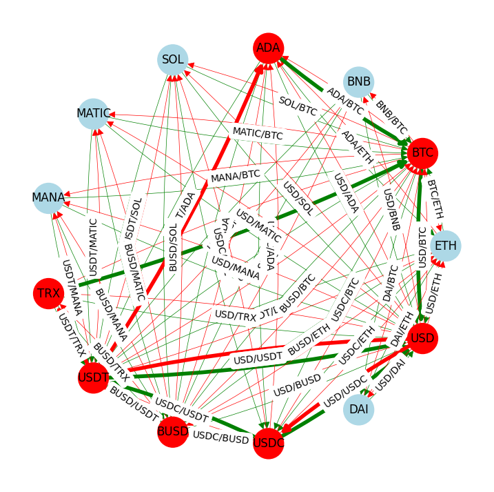
We next illustrate the arbitrage strategy in the graph by marking all the corresponding arcs thicker.

# for each currency we took only one ask and one bid, this is why we are unique between each pair of nodes

# report what orders to issue
for src, dst in m.EDGES:
    if m.z[src, dst]() > 0.0000002:
        order_book_dg.nodes[src]["color"] = "red"
        order_book_dg.nodes[dst]["color"] = "red"
        order_book_dg[src][dst]["width"] = 4

draw_dg(order_book_dg, 0.05)
plt.show()

../../_images/8fe7be5a2fedb472960cc6e8d5a6e7ebef36528ae6ed33a3aa505374e9875be3.png

If we want to be even more precise about the execution of the trading strategy, we can formulate a printout of the list of orders that we, as the counter party to the orders stated in the order book, should issue for our strategy to take place.

# report what orders to issue
print("Trading Summary for the Order Book")
print(f"  Order Book   Type    Capacity         Traded")
for src, dst in m.EDGES:
    if m.z[src, dst]() > 0.0000002:
        kind = order_book_dg.edges[(src, dst)]["kind"]
        s = f"{src:>5s} -> {dst:<5s} {kind} {m.c[src, dst]:12.5f} {m.z[src, dst]():14.5f}"
        s += "  >>>  "
        if kind == "ask":
            base = dst
            quote = src
            symbol = base + "/" + quote
            price = 1.0 / order_book_dg.edges[(src, dst)]["a"]
            volume = m.z[src, dst]() / price
            s += f"sell {volume:15.6f} {symbol:11s} at {price:12.6f}"

        if kind == "bid":
            base = src
            quote = dst
            symbol = base + "/" + quote
            price = order_book_dg.edges[(src, dst)]["a"]
            volume = m.z[src, dst]()
            s += f"buy {volume:16.6f} {symbol:11s} at {price:12.6f}"
        print(s)

Trading Summary for the Order Book
  Order Book   Type    Capacity         Traded
  BTC -> USD   bid      0.00746        0.00004  >>>  buy         0.000042 BTC/USD     at 23373.010000
  ADA -> BTC   bid      2.00000        2.00000  >>>  buy         2.000000 ADA/BTC     at     0.000015
  TRX -> BTC   bid      4.00000        4.00000  >>>  buy         4.000000 TRX/BTC     at     0.000003
 USDT -> ADA   ask    178.28100        0.69750  >>>  sell        2.000000 ADA/USDT    at     0.348750
 USDT -> BUSD  ask 317048.85971    20004.04600  >>>  sell    20012.050820 BUSD/USDT   at     0.999600
 USDT -> TRX   ask    750.05354        0.27732  >>>  sell        4.000000 TRX/USDT    at     0.069330
 USDT -> USD   bid  10407.87000     4958.23550  >>>  buy      4958.235500 USDT/USD    at     1.000000
 BUSD -> USDC  ask 279879.62000    20012.05100  >>>  sell    20012.051000 USDC/BUSD   at     1.000000
 USDC -> USDT  bid 307657.00000    20007.97600  >>>  buy     20007.976000 USDC/USDT   at     1.000100
 USDC -> USD   bid   5050.30000     5050.30000  >>>  buy      5050.300000 USDC/USD    at     0.999900
  USD -> USDT  ask 954935.16397     4953.77430  >>>  sell     4953.278972 USDT/USD    at     1.000100
  USD -> USDC  ask 517682.17000     5046.22570  >>>  sell     5046.225700 USDC/USD    at     1.000000

In the end, we can illustrate the time-journey of our balances in different currencies using time-indexed bar charts.

# display currency balances
balances = pd.DataFrame()
for node in order_book_dg.nodes:
    if sum(m.v[node, t]() for t in m.T0) > 0.0000002:
        for t in m.T0:
            balances.loc[t, node] = m.v[node, t]()

balances.plot(
    kind="bar",
    subplots=True,
    figsize=(8, 10),
    xlabel="Transaction",
    ylabel="Currency Units",
)
plt.gcf().tight_layout()
plt.show()

../../_images/06eb2ef896260feb73fe97d3f472b664ef63288789733cb5e3331e8ddaefce6a.png

Exercises for the reader#

The previous notebook cells made certain assumptions that we need to consider. The first assumption was that there was at most one bid and one ask order between any pair of currencies in an exchange. This assumption was based on the number of orders we downloaded from the online database, but in reality, there may be more orders. How would the presence of multiple orders per pair affect our graph formulation? How can we adjust the MILO formulation to account for this?

Another assumption was that we only traded currencies within one exchange. However, in reality, we can trade across multiple exchanges. How can we modify the graph-based problem formulation to accommodate this scenario?

Further, we have assigned no cost to the number of trades required to implement the strategy produced by optimization. How can the modeled be modified to either minimize the number of trades, or to explicitly include trading costs?

Finally, a tool like this needs to operate in real time. How can this model be incorporated into, say, a streamlit application that could be used to monitor for arbitrage opportunities in real time?

Real Time Downloads of Order Books from an Exchange#

The goal of this notebook was to show how network algorithms and optimization can be utilized to detect arbitrage opportunities within an order book that has been obtained from a cryptocurrency exchange.

The subsequent cell in the notebook utilizes ccxt.exchange.fetch_order_book to obtain the highest bid and lowest ask orders from an exchange for market symbols that meet the criteria of having a minimum in-degree for their base currencies.

def get_order_book(exchange, exchange_dg):
    def get_orders(base, quote, limit=1):
        result = exchange.fetch_order_book("/".join([base, quote]), limit)
        if not result["asks"] or not result["bids"]:
            result = None
        else:
            result["base"], result["quote"] = base, quote
            result["timestamp"] = exchange.milliseconds()
            result["bid_price"], result["bid_volume"] = result["bids"][0]
            result["ask_price"], result["ask_volume"] = result["asks"][0]
        return result

    # fetch order book data and store in a dictionary
    order_book = filter(
        lambda r: r is not None,
        [get_orders(base, quote) for quote, base in exchange_dg.edges()],
    )

    # convert to pandas dataframe
    order_book = pd.DataFrame(order_book)
    order_book["timestamp"] = pd.to_datetime(order_book["timestamp"], unit="ms")

    return order_book[
        [
            "symbol",
            "timestamp",
            "base",
            "quote",
            "bid_price",
            "bid_volume",
            "ask_price",
            "ask_volume",
        ]
    ]


minimum_in_degree = 10

# get graph of market symbols with mininum_in_degree for base currencies
exchange_dg = get_exchange_dg(exchange, minimum_in_degree)

# get order book for all markets in the graph
order_book = get_order_book(exchange, exchange_dg)
order_book_dg = order_book_to_dg(order_book)

# find trades
v0 = 10000.0
m = crypto_model(order_book_dg, T=12, v0=v0)
vT = m.wealth()

print(f"Potential Return = {10000*(vT - v0)/v0:0.3f} basis points")
display(order_book)

Potential Return = 0.000 basis points

	symbol	timestamp	base	quote	bid_price	bid_volume	ask_price	ask_volume
0	ETH/BTC	2023-10-26 10:28:07.688	ETH	BTC	0.0534	1.00000	0.0535	1.01680
1	BTC/USDT	2023-10-26 10:28:07.785	BTC	USDT	34422.5300	0.04934	34450.7000	0.00128
2	ETH/USDT	2023-10-26 10:28:08.017	ETH	USDT	1840.2700	1.07030	1841.6900	2.09630
3	BAT/USDT	2023-10-26 10:28:08.118	BAT	USDT	0.2032	659.00000	0.2044	804.00000
4	ETC/USDT	2023-10-26 10:28:08.213	ETC	USDT	16.5500	6.27000	16.8500	0.10000
...	...	...	...	...	...	...	...	...
143	BTC/USDC	2023-10-26 10:28:29.614	BTC	USDC	34358.6800	0.00504	34467.3700	0.00290
144	ETH/USDC	2023-10-26 10:28:29.712	ETH	USDC	1834.3500	1.11010	1862.0600	0.21520
145	BTC/DAI	2023-10-26 10:28:29.828	BTC	DAI	33763.7400	0.00030	35062.9500	0.00030
146	ETH/DAI	2023-10-26 10:28:30.036	ETH	DAI	1635.0100	0.02700	1872.4900	0.00120
147	USDT/USD	2023-10-26 10:28:30.430	USDT	USD	1.0000	4030.00000	1.0006	620.00000

148 rows × 8 columns

The following cell can be used to download additional order book data sets for testing.

from datetime import datetime
import time

# get graph of market symbols with mininum_in_degree for base currencies
minimum_in_degree = 5
exchange_dg = get_exchange_dg(exchange, minimum_in_degree)

# search time
search_time = 20
timeout = time.time() + search_time

# threshold in basis points
arb_threshold = 1.0

# wait for arbitrage opportunity
print(f"Search for {search_time} seconds.")
while time.time() <= timeout:
    print("Basis points = ", end="")
    order_book = get_order_book(exchange, exchange_dg)
    order_book_dg = order_book_to_dg(order_book)

    v0 = 10000.0
    m = crypto_model(order_book_dg, T=12, v0=10000)
    vT = m.wealth()
    bp = 10000 * (vT - v0) / vT
    print(f"{bp:0.3f}")

    if bp >= arb_threshold:
        print("arbitrage found!")
        fname = f"{exchange} orderbook {datetime.utcnow().strftime('%Y%m%d_%H%M%S')}.csv".replace(
            " ", "_"
        )
        order_book.to_csv(fname)
        print(f"order book saved to: {fname}")

print("Search complete.")

Search for 20 seconds.
Basis points = 0.149
Search complete.

Bibliographic Notes#

Crytocurrency markets are relatively new compared to other markets, and relatively few academic papers are available that specifically address arbitrage on those markets. Early studies, such as the following, reported periods of large, recurrent arbitrage opportunities that exist across exchanges, and that can persist for several days or weeks.

Makarov, I., & Schoar, A. (2020). Trading and arbitrage in cryptocurrency markets. Journal of Financial Economics, 135(2), 293-319.

Subsequent work reports these prices differentials do exist, but only at a fraction of the values previously reported, and only for fleeting periods of time.

Crépellière, T., & Zeisberger, S. (2020). Arbitrage in the Market for Cryptocurrencies. Available at SSRN 3606053. https://papers.ssrn.com/sol3/papers.cfm?abstract_id=3606053

The use of network algorithms to identify cross-exchange arbitrage has appeared in the academic literature, and in numerous web sites demonstrating optimization and network applications. Representative examples are cited below.

Peduzzi, G., James, J., & Xu, J. (2021, September). JACK THE RIPPLER: Arbitrage on the Decentralized Exchange of the XRP Ledger. In 2021 3rd Conference on Blockchain Research & Applications for Innovative Networks and Services (BRAINS) (pp. 1-2). IEEE. https://arxiv.org/pdf/2106.16158.pdf

Bruzgė, R., & Šapkauskienė, A. (2022). Network analysis on Bitcoin arbitrage opportunities. The North American Journal of Economics and Finance, 59, 101562. https://doi.org/10.1016/j.najef.2021.101562

Bruzgė, R., & Šapkauskienė, A. (2022). Dataset for Bitcoin arbitrage in different cryptocurrency exchanges. Data in Brief, 40, 107731.

The work in this notebook is related to materials found in the following web resources.

https://anilpai.medium.com/currency-arbitrage-using-bellman-ford-algorithm-8938dcea56ea

Crypto Trading and Arbitrage Identification Strategies

A more complete analysis of trading and exploiting arbitrage opportunities in decentralized finance markets is available in the following paper and thesis.

Byrne, S. An Exploration of Novel Trading and Arbitrage Methods within Decentralised Finance. https://www.scss.tcd.ie/Donal.OMahony/bfg/202021/StephenByrneDissertation.pdf

Levus, R., Berko, A., Chyrun, L., Panasyuk, V., & Hrubel, M. (2021). Intelligent System for Arbitrage Situations Searching in the Cryptocurrency Market. In CEUR Workshop Proceedings (pp. 407-440). http://ceur-ws.org/Vol-2917/paper32.pdf

In addition to the analysis of arbitrage opportunities, convex optimization may also have an important role in the developing of trading algorithms for crypocurrency exchanges.

Angeris, G., Agrawal, A., Evans, A., Chitra, T., & Boyd, S. (2021). Constant function market makers: Multi-asset trades via convex optimization. arXiv preprint arXiv:2107.12484. https://baincapitalcrypto.com/constant-function-market-makers-multi-asset-trades-via-convex-optimization/ and https://arxiv.org/pdf/2107.12484.pdf