
6.1 Economic Order Quantity#
This notebook demonstrates the reformulation of hyperbolic constraints as SOCO with implementation with pyomo.kernel.conic.quadratic and also the direct modeling of the hyperbolic constraint with pyomo.kernel.conic.rotated_quadratic. The example is familiar to any MBA/business student, and has a significant range of applications including warehouse operations.
Usage notes#
The notebook requires a solver that can handle a conic constraint. Pyomo provides a direct interface to the commercial solvers Gurobi and Mosek that include conic solvers. Other nonlinear solvers may solve this problems using more general techniques that are not specific to conic constraints.
For personal installations of Mosek or Gurobi (free licenses available for academic use), use
mosek_directorgurobi_direct.If you do not have access to the Gurobi or Mosek, you can use the
ipoptsolver. Note, however, thatipoptis a general purpose interior point solver, and does not have algorithms specific to conic problems.
import sys, os

if 'google.colab' in sys.modules:
    %pip install idaes-pse --pre >/dev/null 2>/dev/null
    !idaes get-extensions --to ./bin
    os.environ['PATH'] += ':bin'
    solver = "ipopt"
else:
    solver = "mosek_direct"

import pyomo.kernel as pmo
SOLVER = pmo.SolverFactory(solver)

assert SOLVER.available(), f"Solver {solver} is not available."
The EOQ model#
Classical formulation for a single item#
The economic order quantity (EOQ) is a classical problem in inventory management attributed to Ford Harris (1915). This optimization model aims to identify the order quantity that minimizes the cost of maintaining a specific item in the inventory.
Let \(h\) be the annual cost of holding an item including any financing charges, \(c\) be the fixed cost of placing and receiving an order, and \(d\) be the annual demand. If a quantity \(x\) of the product is ordered, it costs \(c\) to place the order, resulting in a per-item order cost of \(x/c\). Assuming that the demand is uniform in time, it will take \(x/d\) years for the demand to completely deplete the inventory and, therefore, an average item will remain in the inventory for \(x / 2d\) years, incurring a cost \(hx / 2d\). To minimize the average per-item cost, we minimize the function
which, modulo multiplying by \(d\), is equivalent to minimizing the function
The economic order quantity (EOQ) is the value of \(x\) that minimizes \(f(x)\), i.e., the optimal solution of the following optimization problem
Given the rather simple domain, we can derive analytically the solution for the EOQ problem by setting the derivative of \(f(x)\) equal to zero and solving the resulting equation, obtaining
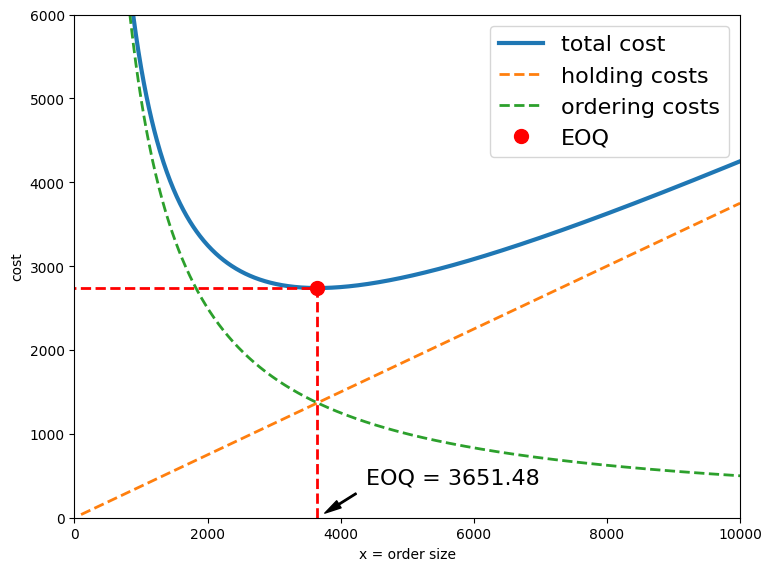
The following chart illustrates the nature of the problem and its analytical solution.
import matplotlib.pyplot as plt
import numpy as np
import pandas as pd

h = 0.75  # cost of holding one item for one year
c = 500.0  # cost of processing one order
d = 10000.0  # annual demand

eoq = np.sqrt(2 * c * d / h)
fopt = np.sqrt(2 * c * d * h)
print(f"Optimal order size = {eoq:0.2f} items with optimal cost {fopt:0.2f}")

x = np.linspace(100, 10000, 1000)
f = h * x / 2 + c * d / x

fig, ax = plt.subplots(figsize=(8, 6))
plt.rcParams.update({"font.size": 16})
ax.plot(x, f, lw=3, label="total cost")
ax.plot(x, h * x / 2, "--", lw=2, label="holding costs")
ax.plot(x, c * d / x, "--", lw=2, label="ordering costs")
ax.set_xlabel("x = order size")
ax.set_ylabel("cost")
ax.plot(eoq, fopt, "ro", ms=10, label="EOQ")
ax.legend(loc="upper right")
ax.annotate(
    f"EOQ = {eoq:0.2f}",
    xy=(eoq, 0),
    xytext=(1.2 * eoq, 0.15 * fopt),
    arrowprops=dict(facecolor="black", shrink=0.15, width=1, headwidth=6),
)
ax.plot([eoq, eoq, 0], [0, fopt, fopt], "r--", lw=2)
ax.set_xlim(0, 10000)
ax.set_ylim(0, 6000)
plt.tight_layout()
plt.show()
Optimal order size = 3651.48 items with optimal cost 2738.61
Reformulating EOQ as a linear objective with hyperbolic constraint#
However, if the problem involved multiple products, an analytical solution would no longer be easily available. For this reason, we need to be able to solve the problem numerically, let us see how.
It can be easily checked that the objective \(f(x)\) is a convex function and therefore, the problem can be solved using any convex optimization solver. It is, however, a special type of convex problem which we shall show in the following reformulation.
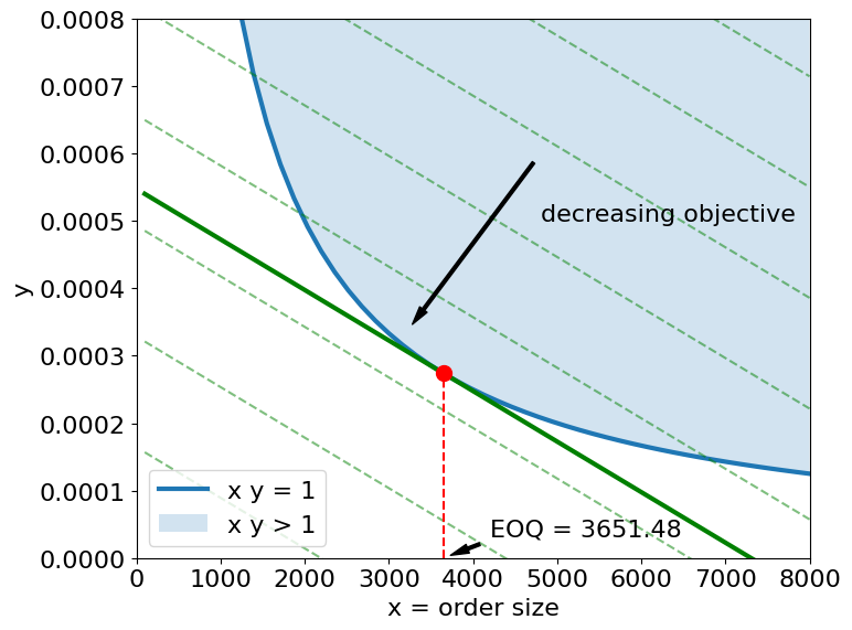
The optimization objective is linearized with the use of a second decision variable \(y = 1/x\). The optimization problem is now a linear objective in two decision variables with a hyperbolic constraint \(xy \geq 1\).
This constraint and the linear contours of the objective function are shown in the following diagrams. The solution of optimization problem occurs at a point where the constraint is tangent to contours of the objective function.
h = 0.75  # cost of holding one item for one year
c = 500.0  # cost of processing one order
d = 10000.0  # annual demand

x = np.linspace(100, 8000)
y = (fopt - h * x / 2) / (c * d)

eoq = np.sqrt(2 * c * d / h)
fopt = np.sqrt(2 * c * d * h)
yopt = (fopt - h * eoq / 2) / (c * d)

fig, ax = plt.subplots(figsize=(8, 6))
ax.plot(x, 1 / x, lw=3, label="x y = 1")
ax.plot(x, (fopt - h * x / 2) / (c * d), "g", lw=3)
for f in fopt * np.linspace(0, 3, 11):
    ax.plot(x, (f - h * x / 2) / (c * d), "g--", alpha=0.5)
ax.plot(eoq, yopt, "ro", ms=10)
ax.annotate(
    f"EOQ = {eoq:0.2f}",
    xy=(eoq, 0),
    xytext=(1.15 * eoq, 0.12 * yopt),
    arrowprops=dict(facecolor="black", shrink=0.15, width=2, headwidth=6),
)

ax.annotate(
    "",
    xytext=(4800, 0.0006),
    xy=(3200, 1 / 3000),
    arrowprops=dict(facecolor="black", shrink=0.05, width=2, headwidth=6),
)
ax.text(4800, 0.0005, "decreasing objective")
ax.fill_between(x, 1 / x, 0.0008, alpha=0.2, label="x y > 1")
ax.plot([eoq, eoq], [0, yopt], "r--")

ax.set_xlim(0, 8000)
ax.set_ylim(0, 0.0008)
ax.set_xlabel("x = order size")
ax.set_ylabel("y")
ax.legend()
plt.tight_layout()
plt.show()
Reformulating the EOQ model with a linear objective and a second order cone constraint#
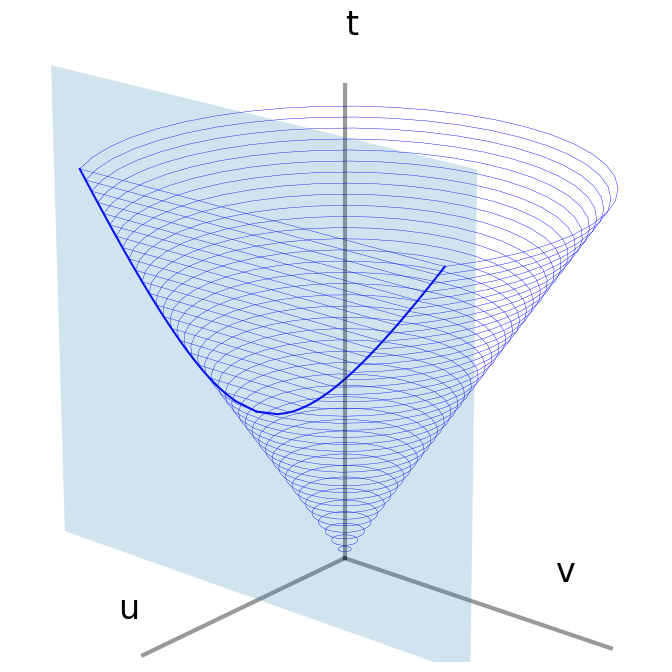
In elementary geometry, a hyperbola can be constructed from the intersection of a linear plane with cone. For this application, the hyperbola described by the constraint \(x y \geq 1\) invites the question of whether there is reformulation of EOQ that includes a cone constraint.
A Lorenz cone is defined by
where the components of are given by \(z = \begin{bmatrix} u \\ v \end{bmatrix}\). The intersection of a plane aligned with the \(t\) axis exactly describes a hyperbola. As described by Lobo, et al. (1998), the correspondence is given by
where the axis in the \(w, x, y\) coordinates is tilted, displaced, and stretched compared to the coordinates shown in the diagram. The exact correspondence to the diagram is given by
The Python code below draws a hyperbola precisely as the intersection of a plane with Lorenz cone.
Let us know rewrite the nonlinear constraint of the EOQ problem. Using the same geometric idea as above and leveraging the non-negativity of both variables, the constraint \(xy \geq 1\) can be reformulated using the following trick:
where we rely on the fact that \(x + y \geq 0\). The final constraint is known as a second-order conic optimization constraint (SOCO constraint). The result is a reformulation of the EOQ problem as a second order conic optimization (SOCO).
import mpl_toolkits.mplot3d.art3d as art3d
from matplotlib.patches import Rectangle

t_max = 4
w = 2
n = 40

fig = plt.figure(figsize=(9, 7))
ax = plt.axes(projection="3d")

for t in np.linspace(0, t_max, n + 1):
    if t < w:
        a = np.linspace(0, 2 * np.pi, 30)
        u = t * np.cos(a)
        v = t * np.sin(a)
        ax.plot3D(u, v, t, "b", lw=0.3)
    else:
        b = np.arccos(w / t)
        a = np.linspace(b, 2 * np.pi - b, 30)
        u = t * np.cos(a)
        v = t * np.sin(a)
        ax.plot3D(u, v, t, "b", lw=0.3)
        ax.plot3D([2, 2], [t * np.sin(b), -t * np.sin(b)], [t, t], "b", lw=0.3)

t = np.linspace(w, t_max)
v = t * np.sin(np.arccos(w / t))
u = w * np.array([1] * len(t))
ax.plot3D(u, v, t, "b")
ax.plot3D(u, -v, t, "b")

ax.plot3D([0, t_max + 0.5], [0, 0], [0, 0], "k", lw=3, alpha=0.4)
ax.plot3D([0, 0], [0, t_max + 1], [0, 0], "k", lw=3, alpha=0.4)
ax.plot3D([0, 0], [0, 0], [0, t_max + 1], "k", lw=3, alpha=0.4)

ax.text3D(t_max + 1, 0, 0.5, "u", fontsize=24)
ax.text3D(0, t_max, 0.5, "v", fontsize=24)
ax.text3D(0, 0, t_max + 1.5, "t", fontsize=24)

ax.view_init(elev=20, azim=40)

r = Rectangle((-t_max, 0), 2 * t_max, t_max + 1, alpha=0.2)
ax.add_patch(r)
art3d.pathpatch_2d_to_3d(r, z=w, zdir="x")

ax.grid(False)
ax.axis("off")

ax.set_xlabel("u")
ax.set_ylabel("v")

ax.set_xlim(-3, 3)
ax.set_ylim(-3, 3)
ax.set_zlim(1, 4)
plt.tight_layout()
plt.show()
Pyomo modeling with conic.quadratic#
The SOCO formation given above needs to be reformulated one more time to use with the Pyomo conic.quadratic constraint. The first step is to introduce rotated coordinates \(t = x+ y\) and \(v = x - y\), and introduce a new variable with fixed value \(u = 2\), to fit the Pyomo model for quadratic constraints,
This version of the model with variables \(t, u, v, x, y\) could be implemented directly in Pyomo with conic.quadratic. However, the model can be further reduced to yield a simpler version of the model.
The EOQ model is now ready to implement with Pyomo and specifically using the Pyomo kernel library. The Pyomo kernel library provides an experimental modeling interface for advanced application development with Pyomo. In particular, the kernel library provides direct support for conic constraints with the Mosek or Gurobi commercial solvers (note that academic licenses are available at no cost).
The Pyomo interface to conic solvers includes six forms for conic constraints. The conic.quadratic constraint is expressed in the form
where the \(x_i\) and \(r\) terms are pyomo.kernel variables. Note the slightly different syntax of the Pyomo kernel commands.
h = 0.75  # cost of holding one item for one year
c = 500.0  # cost of processing one order
d = 10000.0  # annual demand

m = pmo.block()

# define variables for conic constraints
m.u = pmo.variable(lb=0)
m.v = pmo.variable(lb=0)
m.t = pmo.variable(lb=0)

# relationships for conic constraints to decision variables
m.u_eq = pmo.constraint(m.u == 2)
m.q = pmo.conic.quadratic(m.t, [m.u, m.v])

# linear objective
m.eoq = pmo.objective(((h + 2 * c * d) * m.t + (h - 2 * c * d) * m.v) / 4)

# solve
SOLVER.solve(m)

# solution
print(f"\nEOQ = {(m.t() + m.v())/2:0.2f}")
EOQ = 3654.48
The .as_domain() method simplifie the Pyomo model#
pyomo.kernel provides additional support for conic solvers with the .as_domain() method that be applied to the conic solver interfaces. Adding .as_domain allows use of constants, linear expressions, or None in place of Pyomo variables. For this application, this means u does not have to be included as a Pyomo variable and constrained to a fixed value. The required value can simply be inserted directly into constraint specification as demonstrated below.
h = 0.75  # cost of holding one item for one year
c = 500.0  # cost of processing one order
d = 10000.0  # annual demand

m = pmo.block()

# define variables for conic constraints
m.v = pmo.variable(lb=0)
m.t = pmo.variable(lb=0)

# relationships for conic constraints to decision variables
m.q = pmo.conic.quadratic.as_domain(m.t, [2, m.v])

# linear objective
m.eoq = pmo.objective(((h + 2 * c * d) * m.t + (h - 2 * c * d) * m.v) / 4)

# solve
SOLVER.solve(m)

# solution
print(f"\nEOQ = {(m.t() + m.v())/2:0.2f}")
EOQ = 3654.48
Pyomo Modeling with conic.rotated_quadratic#
The need to rotate the natural coordinates of the EOQ problem to fit the programming interface to conic.quadratic is not a big stumbling block, but does raise the question of whether there is a more natural way to express hyperbolic or cone constraints in Pyomo.
pyomo.kernel.conic.rotated_quadratic expresses constraints in the form
This enables a direct a expression of the hyperbolic constraint \(x y \geq 1\) by introducing an auxiliary variable \(z\) with fixed value \(z^2 = 2\) such that
The model to be implemented in Pyomo is now
which is demonstrated below. Note the improvement in accuracy of this calculation compared to the previous solutions. Also note the use of .as_domain() eliminates the need to specify a variable \(z\).
h = 0.75  # cost of holding one time for one year
c = 500.0  # cost of processing one order
d = 10000.0  # annual demand

m = pmo.block()

# define variables for conic constraints
m.x = pmo.variable(lb=0)
m.y = pmo.variable(lb=0)

# conic constraint
m.q = pmo.conic.rotated_quadratic.as_domain(m.x, m.y, [np.sqrt(2)])

# linear objective
m.eoq = pmo.objective(h * m.x / 2 + c * d * m.y)

# solve
SOLVER.solve(m)

# solution
print(f"\nEOQ = {m.x():0.2f}")
EOQ = 3651.48
Extending the EOQ model multiple items with a shared resource#
Solving for the EOQ for a single item using SOCO optimization is using a sledgehammer to swat a fly. However, the problem becomes more interesting for determining economic order quantities when the inventories for multiple items compete for a shared resource in a common warehouse. The shared resource could he financing available to hold inventory, space in a warehouse, or specialized facilities to hold a perishable
where \(h_i\) is the annual holding cost for one unit of item \(i\), \(c_i\) is the cost to place an order and receive delivery for item \(i\), and \(d_i\) is the annual demand. The additional constraint models an allocation of \(b_i\) of the shared resource, and \(b_0\) is the total resource available.
Following the reformulation of the single item model, a variable \(y_i \geq 0\), \(i=1, \dots, n\) is introduced to linearize the objective
Following the discussion above regarding rotated quadratic constraints, auxiliary variables \(z_i\) for \(i=1, \dots, n\) is introduced
The following Pyomo model is a direct implementation of the multi-time EOQ formulation and applied to a hypothetical car parts store that maintains an inventory of tires.
df = pd.DataFrame(
    {
        "all weather": {"h": 1.0, "c": 200, "d": 1300, "b": 3},
        "truck": {"h": 2.8, "c": 250, "d": 700, "b": 8},
        "heavy duty": {"h": 1.2, "c": 200, "d": 500, "b": 5},
        "low cost": {"h": 0.8, "c": 180, "d": 2000, "b": 3},
    }
).T

display(df)
| h | c | d | b | |
|---|---|---|---|---|
| all weather | 1.0 | 200.0 | 1300.0 | 3.0 |
| truck | 2.8 | 250.0 | 700.0 | 8.0 |
| heavy duty | 1.2 | 200.0 | 500.0 | 5.0 |
| low cost | 0.8 | 180.0 | 2000.0 | 3.0 |
def eoq(df, b):
    m = pmo.block()

    m.b = pmo.parameter(b)

    m.I = df.index

    # variable dictionaries
    m.x = pmo.variable_dict()
    for i in m.I:
        m.x[i] = pmo.variable(lb=0)

    m.y = pmo.variable_dict()
    for i in m.I:
        m.y[i] = pmo.variable(lb=0)

    # use a block_dict because .as_domain returns a block
    m.q = pmo.block_dict()
    for i in m.I:
        m.q[i] = pmo.conic.rotated_quadratic.as_domain(m.x[i], m.y[i], [np.sqrt(2)])

    m.b_cap = pmo.constraint(sum(df.loc[i, "b"] * m.x[i] for i in m.I) <= m.b)

    # objective
    m.eoq = pmo.objective(
        sum(
            df.loc[i, "h"] * m.x[i] / 2 + df.loc[i, "c"] * df.loc[i, "d"] * m.y[i]
            for i in m.I
        )
    )

    return m


def eoq_display_results(df, m):
    results = pd.DataFrame(
        [[i, m.x[i](), m.x[i]() * df.loc[i, "b"]] for i in m.I],
        columns=["product", "EOQ", "Space Req'd"],
    ).round(1)
    results.set_index("product", inplace=True)

    display(results)
    results.plot(
        y=["EOQ", "Space Req'd"],
        kind="bar",
        subplots=True,
        layout=(2, 1),
        figsize=(10, 6),
    )


display(df)
m = eoq(df, 4000)
SOLVER.solve(m)  # only works with Mosek
eoq_display_results(df, m)
| h | c | d | b | |
|---|---|---|---|---|
| all weather | 1.0 | 200.0 | 1300.0 | 3.0 |
| truck | 2.8 | 250.0 | 700.0 | 8.0 |
| heavy duty | 1.2 | 200.0 | 500.0 | 5.0 |
| low cost | 0.8 | 180.0 | 2000.0 | 3.0 |
| EOQ | Space Req'd | |
|---|---|---|
| product | ||
| all weather | 306.2 | 918.7 |
| truck | 153.2 | 1225.3 |
| heavy duty | 151.0 | 754.9 |
| low cost | 367.0 | 1101.1 |
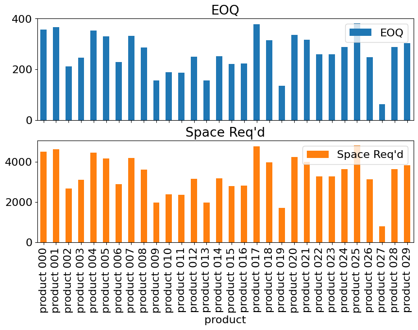
Testing the model on larger problems#
The following cell creates a random EOQ problem of size \(n\) that can be used to test the model formulation and solver.
n = 30
df_large = pd.DataFrame()
df_large["h"] = np.random.uniform(0.5, 2.0, n)
df_large["c"] = np.random.randint(300, 500, n)
df_large["d"] = np.random.randint(100, 5000, n)
df_large["b"] = np.random.uniform(10, 50)
df_large.set_index(pd.Series(f"product {i:03d}" for i in range(n)), inplace=True)

display(df_large)
m = eoq(df_large, 100000)
SOLVER.solve(m)  # only works with Mosek
eoq_display_results(df_large, m)
| h | c | d | b | |
|---|---|---|---|---|
| product 000 | 1.681603 | 464 | 3319 | 12.634027 |
| product 001 | 0.793753 | 409 | 3827 | 12.634027 |
| product 002 | 1.697156 | 481 | 1126 | 12.634027 |
| product 003 | 1.221018 | 325 | 2205 | 12.634027 |
| product 004 | 1.859807 | 463 | 3297 | 12.634027 |
| product 005 | 1.106753 | 354 | 3627 | 12.634027 |
| product 006 | 0.710457 | 343 | 1769 | 12.634027 |
| product 007 | 1.974755 | 331 | 4073 | 12.634027 |
| product 008 | 0.877687 | 493 | 1956 | 12.634027 |
| product 009 | 0.997376 | 302 | 957 | 12.634027 |
| product 010 | 1.794900 | 300 | 1436 | 12.634027 |
| product 011 | 0.756376 | 342 | 1190 | 12.634027 |
| product 012 | 1.923401 | 385 | 1988 | 12.634027 |
| product 013 | 0.534267 | 459 | 618 | 12.634027 |
| product 014 | 0.862266 | 331 | 2230 | 12.634027 |
| product 015 | 1.965372 | 379 | 1582 | 12.634027 |
| product 016 | 1.920569 | 396 | 1554 | 12.634027 |
| product 017 | 1.980645 | 364 | 4836 | 12.634027 |
| product 018 | 0.980492 | 467 | 2497 | 12.634027 |
| product 019 | 1.668067 | 498 | 444 | 12.634027 |
| product 020 | 1.557842 | 434 | 3149 | 12.634027 |
| product 021 | 1.612942 | 396 | 3058 | 12.634027 |
| product 022 | 0.688355 | 492 | 1602 | 12.634027 |
| product 023 | 0.819011 | 471 | 1661 | 12.634027 |
| product 024 | 0.501004 | 452 | 2109 | 12.634027 |
| product 025 | 1.126619 | 405 | 4256 | 12.634027 |
| product 026 | 1.956824 | 434 | 1741 | 12.634027 |
| product 027 | 1.883912 | 402 | 124 | 12.634027 |
| product 028 | 1.908922 | 449 | 2276 | 12.634027 |
| product 029 | 1.789168 | 435 | 2586 | 12.634027 |
| EOQ | Space Req'd | |
|---|---|---|
| product | ||
| product 000 | 356.3 | 4501.3 |
| product 001 | 365.9 | 4623.4 |
| product 002 | 211.2 | 2668.6 |
| product 003 | 245.4 | 3100.1 |
| product 004 | 353.4 | 4465.2 |
| product 005 | 329.2 | 4159.6 |
| product 006 | 228.2 | 2883.7 |
| product 007 | 331.4 | 4186.4 |
| product 008 | 286.7 | 3622.4 |
| product 009 | 156.6 | 1978.1 |
| product 010 | 188.0 | 2375.2 |
| product 011 | 186.8 | 2359.4 |
| product 012 | 249.9 | 3157.6 |
| product 013 | 156.7 | 1979.2 |
| product 014 | 250.9 | 3170.3 |
| product 015 | 221.0 | 2792.4 |
| product 016 | 224.1 | 2831.5 |
| product 017 | 378.6 | 4783.1 |
| product 018 | 314.6 | 3974.7 |
| product 019 | 135.0 | 1706.1 |
| product 020 | 336.5 | 4251.2 |
| product 021 | 316.4 | 3997.2 |
| product 022 | 260.3 | 3288.2 |
| product 023 | 258.6 | 3266.8 |
| product 024 | 287.4 | 3630.8 |
| product 025 | 381.3 | 4817.6 |
| product 026 | 248.2 | 3135.2 |
| product 027 | 63.8 | 806.5 |
| product 028 | 288.9 | 3649.7 |
| product 029 | 303.8 | 3838.6 |
Bibliographic notes#
The original formulation and solution of the economic order quantity problem is attributed to Ford Harris, but in a curious twist has been cited incorrectly since 1931. The correct citation is:
Harris, F. W. (1915). Operations and Cost (Factory Management Series). A. W. Shaw Company, Chap IV, pp.48-52. Chicago.
Harris later developed an extensive consulting business and the concept has become embedded in business practice for over 100 years. Harris’s single item model was later extended to multiple items sharing a resource constraint. There may be earlier citations, but this model is generally attributed to Ziegler (1982):
Ziegler, H. (1982). Solving certain singly constrained convex optimization problems in production planning. Operations Research Letters, 1(6), 246-252. https://www.sciencedirect.com/science/article/abs/pii/016763778290030X
Bretthauer, K. M., & Shetty, B. (1995). The nonlinear resource allocation problem. Operations research, 43(4), 670-683. https://www.jstor.org/stable/171693?seq=1
Reformulation of the multi-item EOQ model as a conic optimization problem is attributed to Kuo and Mittleman (2004) using techniques described by Lobo, et al. (1998):
Kuo, Y. J., & Mittelmann, H. D. (2004). Interior point methods for second-order cone programming and OR applications. Computational Optimization and Applications, 28(3), 255-285. https://link.springer.com/content/pdf/10.1023/B:COAP.0000033964.95511.23.pdf
Lobo, M. S., Vandenberghe, L., Boyd, S., & Lebret, H. (1998). Applications of second-order cone programming. Linear algebra and its applications, 284(1-3), 193-228. https://web.stanford.edu/~boyd/papers/pdf/socp.pdf
The multi-item model has been used didactically many times since 2004. These are representative examples
Letchford, A. N., & Parkes, A. J. (2018). A guide to conic optimisation and its applications. RAIRO-Operations Research, 52(4-5), 1087-1106. http://www.cs.nott.ac.uk/~pszajp/pubs/conic-guide.pdf
El Ghaoui, Laurent (2018). Lecture notes on Optimization Models. https://inst.eecs.berkeley.edu/~ee127/fa19/Lectures/12_socp.pdf
Mosek Modeling Cookbook, section 3.3.5. https://docs.mosek.com/modeling-cookbook/cqo.html.
Appendix: Formulation with SOCO constraints#
Pyomo’s facility for directly handling hyperbolic constraints bypasses the need to formulate SOCO constraints for the multi-item model. For completeness, however, that development is included here.
As a short cut to reformulating the model with conic constraints, note that a “completion of square” gives the needed substitutions
The multi-item EOQ model is now written with conic constraints
Variables \(t_i\), \(u_i\), and \(v_i\) are introduced t complete the reformulation for implementation with Pyomo/Mosek.